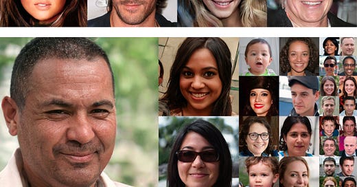
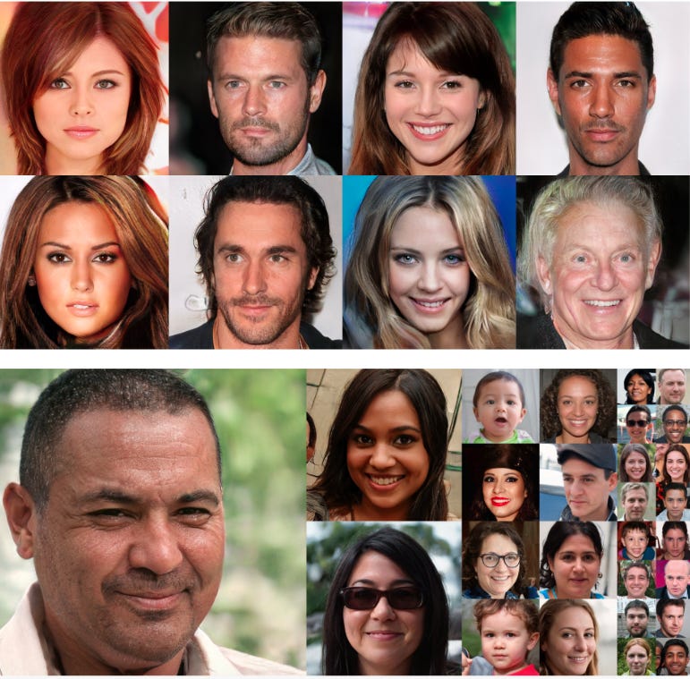
Most of us in data science has seen a lot of AI-generated people in recent times, whether it be in papers, blogs, or videos. We’ve reached a stage where it’s becoming increasingly difficult to distinguish between actual human faces and faces generated by artificial intelligence . However, with the currently available machine learning toolkits, creating these images yourself is not as difficult as you might think.
In my view, GANs will change the way we generate video games and special effects. Using this approach, we could create realistic textures or characters on demand.
So in this post, we’re going to look at the generative adversarial networks behind AI-generated images, and help you to understand how to create and build your similar application with PyTorch. We’ll try to keep the post as intuitive as possible for those of you just starting out, but we’ll try not to dumb it down too much.
At the end of this article, you’ll have a solid understanding of how General Adversarial Networks (GANs) work, and how to build your own.
Task Overview
In this post, we will create unique anime characters using the Anime Face Dataset . It is a dataset consisting of 63,632 high-quality anime faces in a number of styles. It’s a good starter dataset because it’s perfect for our goal.
We will be using Deep Convolutional Generative Adversarial Networks (DC-GANs) for our project. Though we’ll be using it to generate the faces of new anime characters, DC-GANs can also be used to create modern fashion styles , general content creation, and sometimes for data augmentation as well.
But before we get into the coding, let’s take a quick look at how GANs work.
INTUITION: Brief Intro to GANs for Generating Fake Images
GANs typically employ two dueling neural networks to train a computer to learn the nature of a dataset well enough to generate convincing fakes. One of these Neural Networks generates fakes (the generator), and the other tries to classify which images are fake (the discriminator). These networks improve over time by competing against each other.
Perhaps imagine the generator as a robber and the discriminator as a police officer. The more the robber steals, the better he gets at stealing things. But at the same time, the police officer also gets better at catching the thief. Well, in an ideal world, anyway.
The losses in these neural networks are primarily a function of how the other network performs:
Discriminator network loss is a function of generator network quality: Loss is high for the discriminator if it gets fooled by the generator’s fake images.
Generator network loss is a function of discriminator network quality: Loss is high if the generator is not able to fool the discriminator.
In the training phase, we train our discriminator and generator networks sequentially, intending to improve performance for both. The end goal is to end up with weights that help the generator to create realistic-looking images. In the end, we’ll use the generator neural network to generate high-quality fake images from random noise***.***
The Generator architecture
One of the main problems we face when working with GANs is that the training is not very stable. So we have to come up with a generator architecture that solves our problem and also results in stable training. The diagram below is taken from the paper Unsupervised Representation Learning with Deep Convolutional Generative Adversarial Networks , which explains the DC-GAN generator architecture.
Though it might look a little bit confusing, essentially you can think of a generator neural network as a black box which takes as input a 100 dimension normally generated vector of numbers and gives us an image:
So how do we create such an architecture? Below, we use a dense layer of size 4x4x1024 to create a dense vector out of the 100-d vector. We then reshape the dense vector in the shape of an image of 4×4 with 1024 filters, as shown in the following figure:
Note that we don’t have to worry about any weights right now as the network itself will learn those during training.
Once we have the 1024 4×4 maps, we do upsampling using a series of transposed convolutions, which after each operation doubles the size of the image and halves the number of maps. In the last step, however, we don’t halve the number of maps. We reduce the maps to 3 for each RGB channel since we need three channels for the output image.
Now, What are Transpose convolutions?
Put simply, transposing convolutions provides us with a way to upsample images. In a convolution operation, we try to go from a 4×4 image to a 2×2 image. But when we transpose convolutions, we convolve from 2×2 to 4×4 as shown in the following figure:
Some of you may already know that unpooling is commonly used for upsampling input feature maps in convolutional neural networks (CNN). So why don’t we use unpooling here?
The reason comes down to the fact that unpooling does not involve any learning. However, transposed convolution is learnable, so it’s preferred. Later in the article, we’ll see how the parameters can be learned by the generator.
The Discriminator architecture
Now that we’ve covered the generator architecture, let’s look at the discriminator as a black box. In practice, it contains a series of convolutional layers with a dense layer at the end to predict if an image is fake or not. You can see an example in the figure below:
Every image convolutional neural network works by taking an image as input, and predicting if it is real or fake using a sequence of convolutional layers.
Data preprocessing and visualization
Before going any further with our training, we preprocess our images to a standard size of 64x64x3. We will also need to normalize the image pixels before we train our GAN. You can see the process in the code below, which I’ve commented on for clarity.
# Root directory for dataset
dataroot = "anime_images/"
# Number of workers for dataloader
workers = 2
# Batch size during training
batch_size = 128
# Spatial size of training images. All images will be resized to this size using a transformer.
image_size = 64
# Number of channels in the training images. For color images this is 3
nc = 3
# We can use an image folder dataset the way we have it setup.
# Create the dataset
dataset = datasets.ImageFolder(root=dataroot,
transform=transforms.Compose([
transforms.Resize(image_size),
transforms.CenterCrop(image_size),
transforms.ToTensor(),
transforms.Normalize((0.5, 0.5, 0.5), (0.5, 0.5, 0.5)),
]))
# Create the dataloader
dataloader = torch.utils.data.DataLoader(dataset, batch_size=batch_size,
shuffle=True, num_workers=workers)
# Decide which device we want to run on
device = torch.device("cuda:0" if (torch.cuda.is_available() and ngpu > 0) else "cpu")
# Plot some training images
real_batch = next(iter(dataloader))
plt.figure(figsize=(8,8))
plt.axis("off")
plt.title("Training Images")
plt.imshow(np.transpose(vutils.make_grid(real_batch[0].to(device)[:64], padding=2, normalize=True).cpu(),(1,2,0)))
The resultant output of the code is as follows:
Implementation of DCGAN
This is the part where we define our DCGAN. We will be defining our noise generator function, Generator architecture, and Discriminator architecture.
Generating noise vector for Generator
We need to generate the noise which we want to convert to an image using our generator architecture.
We use a normal distribution
to generate the noise vector:
nz = 100
noise = torch.randn(64, nz, 1, 1, device=device)
Generator architecture
The generator is the most crucial part of the GAN. Here, we’ll create a generator by adding some transposed convolution layers to upsample the noise vector to an image. You’ll notice that this generator architecture is not the same as the one given in the DC-GAN paper I linked above.
In order to make it a better fit for our data, I had to make some architectural changes. I added a convolution layer in the middle and removed all dense layers from the generator architecture to make it fully convolutional.
I also used a lot of Batchnorm layers and leaky ReLU activation. The following code block is the function I will use to create the generator:
# Size of feature maps in generator
ngf = 64
# Number of channels in the training images. For color images this is 3
nc = 3
# Size of z latent vector (i.e. size of generator input noise)
nz = 100
class Generator(nn.Module):
def __init__(self, ngpu):
super(Generator, self).__init__()
self.ngpu = ngpu
self.main = nn.Sequential(
# input is noise, going into a convolution
# Transpose 2D conv layer 1.
nn.ConvTranspose2d( nz, ngf * 8, 4, 1, 0, bias=False),
nn.BatchNorm2d(ngf * 8),
nn.ReLU(True),
# Resulting state size - (ngf*8) x 4 x 4 i.e. if ngf= 64 the size is 512 maps of 4x4
# Transpose 2D conv layer 2.
nn.ConvTranspose2d(ngf * 8, ngf * 4, 4, 2, 1, bias=False),
nn.BatchNorm2d(ngf * 4),
nn.ReLU(True),
# Resulting state size -(ngf*4) x 8 x 8 i.e 8x8 maps
# Transpose 2D conv layer 3.
nn.ConvTranspose2d( ngf * 4, ngf * 2, 4, 2, 1, bias=False),
nn.BatchNorm2d(ngf * 2),
nn.ReLU(True),
# Resulting state size. (ngf*2) x 16 x 16
# Transpose 2D conv layer 4.
nn.ConvTranspose2d( ngf * 2, ngf, 4, 2, 1, bias=False),
nn.BatchNorm2d(ngf),
nn.ReLU(True),
# Resulting state size. (ngf) x 32 x 32
# Final Transpose 2D conv layer 5 to generate final image.
# nc is number of channels - 3 for 3 image channel
nn.ConvTranspose2d( ngf, nc, 4, 2, 1, bias=False),
# Tanh activation to get final normalized image
nn.Tanh()
# Resulting state size. (nc) x 64 x 64
)
def forward(self, input):
''' This function takes as input the noise vector'''
return self.main(input)
Now we can instantiate the model using the generator class. We are keeping the default weight initializer for PyTorch even though the paper says to initialize the weights using a mean of 0 and std dev of 0.2. The default weights initializer from Pytorch is more than good enough for our project.
# Create the generator
netG = Generator(ngpu).to(device)
# Handle multi-gpu if desired
if (device.type == 'cuda') and (ngpu > 1):
netG = nn.DataParallel(netG, list(range(ngpu)))
# Print the model
print(netG)
We can see the final generator model:
The Discriminator architecture
Here is the discriminator architecture where I use a series of convolutional layers and a dense layer at the end to predict if an image is fake or not.
# Number of channels in the training images. For color images this is 3
nc = 3
# Size of feature maps in discriminator
ndf = 64
class Discriminator(nn.Module):
def __init__(self, ngpu):
super(Discriminator, self).__init__()
self.ngpu = ngpu
self.main = nn.Sequential(
# input is (nc) x 64 x 64
nn.Conv2d(nc, ndf, 4, 2, 1, bias=False),
nn.LeakyReLU(0.2, inplace=True),
# state size. (ndf) x 32 x 32
nn.Conv2d(ndf, ndf * 2, 4, 2, 1, bias=False),
nn.BatchNorm2d(ndf * 2),
nn.LeakyReLU(0.2, inplace=True),
# state size. (ndf*2) x 16 x 16
nn.Conv2d(ndf * 2, ndf * 4, 4, 2, 1, bias=False),
nn.BatchNorm2d(ndf * 4),
nn.LeakyReLU(0.2, inplace=True),
# state size. (ndf*4) x 8 x 8
nn.Conv2d(ndf * 4, ndf * 8, 4, 2, 1, bias=False),
nn.BatchNorm2d(ndf * 8),
nn.LeakyReLU(0.2, inplace=True),
# state size. (ndf*8) x 4 x 4
nn.Conv2d(ndf * 8, 1, 4, 1, 0, bias=False),
nn.Sigmoid()
)
def forward(self, input):
return self.main(input)
Now we can instantiate the discriminator exactly as we did the generator.
# Create the Discriminator
netD = Discriminator(ngpu).to(device)
# Handle multi-gpu if desired
if (device.type == 'cuda') and (ngpu > 1):
netD = nn.DataParallel(netD, list(range(ngpu)))
# Print the model
print(netD)
Here is the architecture of the discriminator:
Training
Understanding how the training works in GAN is essential. It’s interesting, too; we can see how training the generator and discriminator together improves them both at the same time.
Now that we have our discriminator and generator models, next we need to initialize separate optimizers for them.
# Initialize BCELoss function
criterion = nn.BCELoss()
# Create batch of latent vectors that we will use to visualize
# the progression of the generator
fixed_noise = torch.randn(64, nz, 1, 1, device=device)
# Establish convention for real and fake labels during training
real_label = 1.
fake_label = 0.
# Setup Adam optimizers for both G and D
# Learning rate for optimizers
lr = 0.0002
# Beta1 hyperparam for Adam optimizers
beta1 = 0.5
optimizerD = optim.Adam(netD.parameters(), lr=lr, betas=(beta1, 0.999))
optimizerG = optim.Adam(netG.parameters(), lr=lr, betas=(beta1, 0.999))
The Training Loop
This is the main area where we need to understand how the blocks we’ve created will assemble and work together.
# Lists to keep track of progress/Losses
img_list = []
G_losses = []
D_losses = []
iters = 0
# Number of training epochs
num_epochs = 50
# Batch size during training
batch_size = 128
print("Starting Training Loop...")
# For each epoch
for epoch in range(num_epochs):
# For each batch in the dataloader
for i, data in enumerate(dataloader, 0):
############################
# (1) Update D network: maximize log(D(x)) + log(1 - D(G(z)))
# Here we:
# A. train the discriminator on real data
# B. Create some fake images from Generator using Noise
# C. train the discriminator on fake data
###########################
# Training Discriminator on real data
netD.zero_grad()
# Format batch
real_cpu = data[0].to(device)
b_size = real_cpu.size(0)
label = torch.full((b_size,), real_label, device=device)
# Forward pass real batch through D
output = netD(real_cpu).view(-1)
# Calculate loss on real batch
errD_real = criterion(output, label)
# Calculate gradients for D in backward pass
errD_real.backward()
D_x = output.mean().item()
## Create a batch of fake images using generator
# Generate noise to send as input to the generator
noise = torch.randn(b_size, nz, 1, 1, device=device)
# Generate fake image batch with G
fake = netG(noise)
label.fill_(fake_label)
# Classify fake batch with D
output = netD(fake.detach()).view(-1)
# Calculate D's loss on the fake batch
errD_fake = criterion(output, label)
# Calculate the gradients for this batch
errD_fake.backward()
D_G_z1 = output.mean().item()
# Add the gradients from the all-real and all-fake batches
errD = errD_real + errD_fake
# Update D
optimizerD.step()
############################
# (2) Update G network: maximize log(D(G(z)))
# Here we:
# A. Find the discriminator output on Fake images
# B. Calculate Generators loss based on this output. Note that the label is 1 for generator.
# C. Update Generator
###########################
netG.zero_grad()
label.fill_(real_label) # fake labels are real for generator cost
# Since we just updated D, perform another forward pass of all-fake batch through D
output = netD(fake).view(-1)
# Calculate G's loss based on this output
errG = criterion(output, label)
# Calculate gradients for G
errG.backward()
D_G_z2 = output.mean().item()
# Update G
optimizerG.step()
# Output training stats every 50th Iteration in an epoch
if i % 1000 == 0:
print('[%d/%d][%d/%d]\tLoss_D: %.4f\tLoss_G: %.4f\tD(x): %.4f\tD(G(z)): %.4f / %.4f'
% (epoch, num_epochs, i, len(dataloader),
errD.item(), errG.item(), D_x, D_G_z1, D_G_z2))
# Save Losses for plotting later
G_losses.append(errG.item())
D_losses.append(errD.item())
# Check how the generator is doing by saving G's output on a fixed_noise vector
if (iters % 250 == 0) or ((epoch == num_epochs-1) and (i == len(dataloader)-1)):
#print(iters)
with torch.no_grad():
fake = netG(fixed_noise).detach().cpu()
img_list.append(vutils.make_grid(fake, padding=2, normalize=True))
iters += 1
It may seem complicated, but I’ll break down the code above step by step in this section. The main steps in every training iteration are:
Step 1: Sample a batch of normalized images from the dataset
for i, data in enumerate(dataloader, 0):
Step 2: Train discriminator using generator images(Fake images) and real normalized images(Real Images) and their labels.
# Training Discriminator on real data
netD.zero_grad()
# Format batch
real_cpu = data[0].to(device)
b_size = real_cpu.size(0)
label = torch.full((b_size,), real_label, device=device)
# Forward pass real batch through D
output = netD(real_cpu).view(-1)
# Calculate loss on real batch
errD_real = criterion(output, label)
# Calculate gradients for D in backward pass
errD_real.backward()
D_x = output.mean().item() ## Create a batch of fake images
# Generate noise to send as input to the generator
noise = torch.randn(b_size, nz, 1, 1, device=device)
# Generate fake image batch with G
fake = netG(noise)
label.fill_(fake_label)
# Classify fake batch with D
output = netD(fake.detach()).view(-1)
# Calculate D's loss on the fake batch
errD_fake = criterion(output, label)
# Calculate the gradients for this batch
errD_fake.backward()
D_G_z1 = output.mean().item()
# Add the gradients from the all-real and all-fake batches
errD = errD_real + errD_fake
# Update D
optimizerD.step()
Step 3: Backpropagate the errors through the generator by computing the loss gathered from discriminator output on fake images as the input and 1’s as the target while keeping the discriminator as untrainable — This ensures that the loss is higher when the generator is not able to fool the discriminator. You can check it yourself like so: if the discriminator gives 0 on the fake image, the loss will be high i.e., BCELoss(0,1).
netG.zero_grad()
label.fill_(real_label)
# fake labels are real for generator cost
output = netD(fake).view(-1)
# Calculate G's loss based on this output
errG = criterion(output, label)
# Calculate gradients for G
errG.backward()
D_G_z2 = output.mean().item()
# Update G
optimizerG.step()
We repeat the steps using the for loop to end up with a good discriminator and generator.
Results
The final output of our generator can be seen below. The GAN generates pretty good images for our content editor friends to work with.
The images might be a little crude, but still, this project was a starter for our GAN journey. The field is constantly advancing with better and more complex GAN architectures, so we’ll likely see further increases in image quality from these architectures. Also, keep in mind that these images are generated from a noise vector only: this means the input is some noise, and the output is an image. It’s quite incredible.
ALL THESE IMAGES ARE FAKE
1. Loss over the training period
Here is the graph generated for the losses. We can see that the GAN Loss is decreasing on average, and the variance is also decreasing as we do more steps. It’s possible that training for even more iterations would give us even better results.
plt.figure(figsize=(10,5))
plt.title("Generator and Discriminator Loss During Training")
plt.plot(G_losses,label="G")
plt.plot(D_losses,label="D")
plt.xlabel("iterations")
plt.ylabel("Loss")
plt.legend()
plt.show()
2. Image Animation at every 250th Iteration in Jupyter Notebook
We can choose to see the output as an animation using the below code:
#%%capture
fig = plt.figure(figsize=(8,8))
plt.axis("off")
ims = [[plt.imshow(np.transpose(i,(1,2,0)), animated=True)] for i in img_list]
ani = animation.ArtistAnimation(fig, ims, interval=1000, repeat_delay=1000, blit=True)HTML(ani.to_jshtml())
You can choose to save an animation object as a gif as well if you want to send them to some friends.
ani.save('animation.gif', writer='imagemagick',fps=5)
Image(url='animation.gif')
3. Image generated at every 200 Iter
Given below is the code to generate some images at different training steps. As we can see, as the number of steps increases, the images are getting better.
# create a list of 16 images to show
every_nth_image = np.ceil(len(img_list)/16)
ims = [np.transpose(img,(1,2,0)) for i,img in enumerate(img_list)if i%every_nth_image==0]
print("Displaying generated images")
# You might need to change grid size and figure size here according to num images.
plt.figure(figsize=(20,20))
gs1 = gridspec.GridSpec(4, 4)
gs1.update(wspace=0, hspace=0)
step = 0
for i,image in enumerate(ims):
ax1 = plt.subplot(gs1[i])
ax1.set_aspect('equal')
fig = plt.imshow(image)
# you might need to change some params here
fig = plt.text(7,30,"Step: "+str(step),bbox=dict(facecolor='red', alpha=0.5),fontsize=12)
plt.axis('off')
fig.axes.get_xaxis().set_visible(False)
fig.axes.get_yaxis().set_visible(False)
step+=int(250*every_nth_image)
#plt.tight_layout()
plt.savefig("GENERATEDimage.png",bbox_inches='tight',pad_inches=0)
plt.show()
Given below is the result of the GAN at different time steps:
Conclusion
In this post, we covered the basics of GANs for creating fairly believable fake images. We hope you now have an understanding of generator and discriminator architecture for DC-GANs, and how to build a simple DC-GAN to generate anime images from scratch.
Though this model is not the most perfect anime face generator, using it as a base helps us to understand the basics of generative adversarial networks, which in turn can be used as a stepping stone to more exciting and complex GANs as we move forward.
Look at it this way, as long as we have the training data at hand, we now have the ability to conjure up realistic textures or characters on demand. That is no small feat.
For a closer look at the code for this post, please visit my GitHub repository where you can find the code for this post as well as all my posts.
If you want to know more about deep learning applications and use cases, take a look at the Sequence Models course in the Deep Learning Specialization by Andrew Ng. Andrew is a great instructor, and this course is excellent too.
I am going to be writing more of such posts in the future too. Let me know what you think about the series. Follow me up at Medium or Subscribe to my blog .
Also, a small disclaimer — There might be some affiliate links in this post to relevant resources, as sharing knowledge is never a bad idea.
This post was first published here