Demystifying Object Detection and Instance Segmentation for Data Scientists

I like deep learning a lot but Object Detection is something that doesn’t come easily to me.

And Object detection is important and does have its uses. Most common of them being self-driving cars, medical imaging and face detection.

It is definitely a hard problem to solve. And with so many moving parts and new concepts introduced over the long history of this problem, it becomes even harder to understand.

This post is about distilling that history into an easy explanation and explaining the gory details for Object Detection and Instance Segmentation.

Introduction

We all know about the image classification problem. Given an image can you find out the class the image belongs to?

We can solve any new image classification problem with ConvNets and Transfer Learning using pre-trained nets.

ConvNet as fixed feature extractor. Take a ConvNet pretrained on ImageNet, remove the last fully-connected layer (this layer’s outputs are the 1000 class scores for a different task like ImageNet), then treat the rest of the ConvNet as a fixed feature extractor for the new dataset. In an AlexNet, this would compute a 4096-D vector for every image that contains the activations of the hidden layer immediately before the classifier. We call these features CNN codes. It is important for performance that these codes are ReLUd (i.e. thresholded at zero) if they were also thresholded during the training of the ConvNet on ImageNet (as is usually the case). Once you extract the 4096-D codes for all images, train a linear classifier (e.g. Linear SVM or Softmax classifier) for the new dataset.

But there are lots of other interesting problems in the Image domain:

Source

These problems can be divided into 4 major buckets. In the next few lines I would try to explain each of these problems concisely before we take a deeper dive:

1. Semantic Segmentation: Given an image, can we classify each pixel as belonging to a particular class?

2. Classification+Localization: We were able to classify an image as a cat. Great. Can we also get the location of the said cat in that image by drawing a bounding box around the cat? Here we assume that there is a fixed number of objects(commonly 1) in the image.

3. Object Detection: A More general case of the Classification+Localization problem. In a real-world setting, we don’t know how many objects are in the image beforehand. So can we detect all the objects in the image and draw bounding boxes around them?

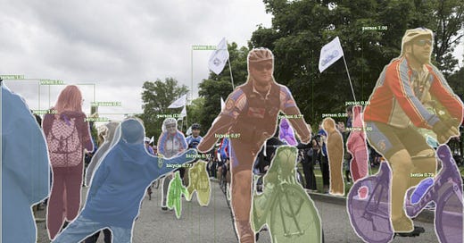
4. Instance Segmentation: Can we create masks for each individual object in the image? It is different from semantic segmentation. How? If you look in the 4th image on the top, we won’t be able to distinguish between the two dogs using semantic segmentation procedure as it would sort of merge both the dogs together.

As you can see all the problems have something of a similar flavour but a little different than each other. In this post, I will focus mainly on Object Detection and Instance segmentation as they are the most interesting.I will go through the 4 most famous techniques for object detection and how they improved with time and new ideas.

Classification+Localization

So lets first try to understand how we can solve the problem when we have a single object in the image. How to solve the Classification+Localization case.

💡 Treat localization as a regression problem!

Input Data

Lets first talk about what sort of data such sort of model expects. Normally in an image classification setting, we used to have data in the form (X,y) where X is the image and y used to be the class label.

In the Classification+Localization setting, we will have data normally in the form (X,y), where X is still the image and y is an array containing (class_label, x,y,w,h) where,

x = bounding box top left corner x-coordinate

y = bounding box top left corner y-coordinate

w = width of the bounding box in pixels

h = height of the bounding box in pixels

Model

So in this setting, we create a multi-output model which takes an image as the input and has (n_labels + 4) output nodes. n_labels nodes for each of the output class and 4 nodes that give the predictions for (x,y,w,h).

Loss

Normally the loss is a weighted sum of the Softmax Loss(from the Classification Problem) and the regression L2 loss(from the bounding box coordinates).

Loss = alpha*Softmax_Loss + (1-alpha)*L2_Loss

Since these two losses would be on a different scale, the alpha hyper-parameter is something that needs to be tuned.

There is one thing I would like to note here. We are trying to do object localization task but we still have our convnets in place here. We are just adding one more output layer to also predict the coordinates of the bounding box and tweaking our loss function.

And herein lies the essence of the whole Deep Learning framework — Stack layers on top of each other, reuse components to create better models, and create architectures to solve your own problem*. And that is what we are going to see a lot going forward.*

Object Detection

So how does this idea of localization using regression get mapped to Object Detection? It doesn’t.

We don’t have a fixed number of objects. So we can’t have 4 outputs denoting, the bounding box coordinates.

One naive idea could be to apply CNN to many different crops of the image. CNN classifies each crop as an object class or background class. This is intractable. There could be a lot of such crops that you can create.

Region Proposals:

So, if just there was just a method(Normally called Region Proposal Network)which could find some smaller number of cropped regions for us automatically, we could just run our convnet on those regions and be done with object detection. And that is the basic idea behind RCNN-The first major success in object detection.

And that is what selective search (Uijlings et al, “ Selective Search for Object Recognition ”, IJCV 2013) provided.

So what are Region Proposals?

• Find “blobby” image regions that are likely to contain objects

• Relatively fast to run; e.g. Selective Search gives 2000 region proposals in a few seconds on CPU

So, how exactly the region proposals are made?

Selective Search for Object Recognition :

This paper finds regions in two steps.

First, we start with a set of some initial regions using Efficient GraphBased Image Segmentation .

Graph-based image segmentation techniques generally represent the problem in terms of a graph G = (V, E) where each node v ∈ V corresponds to a pixel in the image, and the edges in E connect certain pairs of neighboring pixels.

In this paper they take an approach:

Each edge (vi , vj )∈ E has a corresponding weight w((vi , vj )), which is a non-negative measure of the similarity between neighboring elements vi and vj . In the graph-based approach, a segmentation S is a partition of V into components such that each component (or region) C ∈ S corresponds to a connected component in a graph.

Put simply, they use graph-based methods to find connected components in an image and the edges are made on some measure of similarity between pixels.

As you can see if we create bounding boxes around these masks we will be losing a lot of regions. We want to have the whole baseball player in a single bounding box/frame. We need to somehow group these initial regions. And that is the second step.

For that, the authors of Selective Search for Object Recognition apply the Hierarchical Grouping algorithm to these initial regions. In this algorithm, they merge most similar regions together based on different notions of similarity based on colour, texture, size and fill to provide us with much better region proposals.

1. R-CNN

So now we have our region proposals. How do we exactly use them in R-CNN?

Object detection system overview. Our system (1) takes an input image, (2) extracts around 2000 bottom-up region proposals, (3) computes features for each proposal using a large convolutional neural network (CNN), and then (4) classifies each region using class-specific linear SVM.

Along with this, the authors have also used a class-specific bounding box regressor, that takes:

Input : (Px, Py, Ph, Pw) — the location of the proposed region.

Target: (Gx, Gy, Gh, Gw) — Ground truth labels for the region.

The goal is to learn a transformation that maps the proposed region(P) to the Ground truth box(G)

Training R-CNN

What is the input to an RCNN?

So we have got an image, Region Proposals from the RPN strategy and the ground truths of the labels (labels, ground truth boxes)

Next, we treat all region proposals with ≥ 0.5 IoU(Intersection over Union) overlap with a ground-truth box as a positive training example for that box’s class and the rest as negative. We train class-specific SVM’s

So every region proposal becomes a training example. and the convnet gives a feature vector for that region proposal. We can then train our n-SVMs using the class-specific data.

Test Time R-CNN

At test time we predict detection boxes using class-specific SVMs. We will be getting a lot of overlapping detection boxes at the time of testing. Thus, non-maximum suppression is an integral part of the object detection pipeline.

First, it sorts all detection boxes on the basis of their scores. The detection box M with the maximum score is selected and all other detection boxes with a significant overlap (using a pre-defined threshold) with M are suppressed.

This process is recursively applied on all the remaining boxes until we are left with good bounding boxes only.

Problems with RCNN:

• Training is slow.

• Inference (detection) is slow. 47s / image with VGG16 — Since the Convnet needs to be run many times.

Need for speed. So Fast R-CNN.

2. Fast R-CNN

💡 So the next idea from the same authors: Why not create convolution map of input image and then just select the regions from that convolutional map? Do we really need to run so many convnets? What we can do is run just a single convnet and then apply region proposal crops on the features calculated by the convnet and use a simple SVM/classifier to classify those crops.

Something like:

From Paper : Fig. illustrates the Fast R-CNN architecture. A Fast R-CNN network takes as input an entire image and a set of object proposals. The network first processes the whole image with several convolutional (conv) and max pooling layers to produce a conv feature map. Then, for each object proposal a region of interest (RoI) pooling layer extracts a fixed-length feature vector from the feature map. Each feature vector is fed into a sequence of fully connected (fc) layers that finally branch into two sibling output layers: one that produces softmax probability estimates over K object classes plus a catch-all “background” class and another layer that outputs four real-valued numbers for each of the K object classes. Each set of 4 values encodes refined bounding-box positions for one of the K classes.

💡Idea

So the basic idea is to have to run the convolution only once in the image rather than so many convolution networks in R-CNN. Then we can map the ROI proposals using some method and filter the last convolution layer and just run a final classifier on that.

This idea depends a little upon the architecture of the model that gets used too.

So the architecture that the authors have proposed is:

We experiment with three pre-trained ImageNet [4] networks, each with five max pooling layers and between five and thirteen conv layers (see Section 4.1 for network details). When a pre-trained network initializes a Fast R-CNN network, it undergoes three transformations. First, the last max pooling layer is replaced by a RoI pooling layer that is configured by setting H and W to be compatible with the net’s first fully connected layer (e.g., H = W = 7 for VGG16). Second, the network’s last fully connected layer and softmax (which were trained for 1000-way ImageNet classification) are replaced with the two sibling layers described earlier (a fully connected layer and softmax over K + 1 categories and category-specific bounding-box regressors). Third, the network is modified to take two data inputs: a list of images and a list of RoIs in those images.

Don’t worry if you don’t understand the above. This obviously is a little confusing, so let us break this down. But for that, we need to see VGG16 architecture first.

The last pooling layer is 7x7x512. This is the layer the network authors intend to replace by the ROI pooling layers. This pooling layer has got as input the location of the region proposal(xmin_roi,ymin_roi,h_roi,w_roi) and the previous feature map(14x14x512).

Now the location of ROI coordinates is in the units of the input image i.e. 224x224 pixels. But the layer on which we have to apply the ROI pooling operation is 14x14x512.

As we are using VGG, we have transformed the image (224 x 224 x 3) into (14 x 14 x 512) — i.e. the height and width are divided by 16. We can map ROIs coordinates onto the feature map just by dividing them by 16.

In its depth, the convolutional feature map has encoded all the information for the image while maintaining the location of the “things” it has encoded relative to the original image. For example, if there was a red square on the top left of the image and the convolutional layers activate for it, then the information for that red square would still be on the top left of the convolutional feature map.

What is ROI pooling?

Remember that the final classifier runs for each crop. And so each crop needs to be of the same size. And that is what ROI Pooling does.

In the above image, our region proposal is (0,3,5,7) in x,y,w,h format.

We divide that area into 4 regions since we want to have an ROI pooling layer of 2x2. We divide the whole area into buckets by rounding 5/2 and 7/2 and then just do a max-pool.

How do you do ROI-Pooling on Areas smaller than the target size? if region proposal size is 5x5 and ROI pooling layer of size 7x7. If this happens, we resize to 35x35 just by copying 7 times each cell and then max-pooling back to 7x7.

After replacing the pooling layer, the authors also replaced the 1000 layer imagenet classification layer by a fully connected layer and softmax over K + 1 categories(+1 for Background) and category-specific bounding-box regressors.

Training Fast-RCNN

What is the input to a Fast- RCNN?

Pretty much similar to R-CNN: So we have got an image, Region Proposals from the RPN strategy and the ground truths of the labels (labels, ground truth boxes)

Next, we treat all region proposals with ≥ 0.5 IoU(Intersection over Union) overlap with a ground-truth box as a positive training example for that box’s class and the rest as negative. This time we have a dense layer on top, and we use multi-task loss.

So every ROI becomes a training example. The main difference is that there is a concept of multi-task loss:

A Fast R-CNN network has two sibling output layers.

The first outputs a discrete probability distribution (per RoI), p = (p0, . . . , pK), over K + 1 categories. As usual, p is computed by a softmax over the K+1 outputs of a fully connected layer.

The second sibling layer outputs bounding-box regression offsets, t= (tx, ty, tw, th), for each of the K object classes. Each training RoI is labelled with a ground-truth class u and a ground-truth bounding-box regression target v. We use a multi-task loss L on each labelled RoI to jointly train for classification and bounding-box regression

Where Lcls is the softmax classification loss and Lloc is the regression loss. u=0 is for BG class and hence we add to loss only when we have a boundary box for any of the other class.

Problem:

Region proposals are still taking up most of the time. Can we reduce the time taken for Region proposals?

3. Faster-RCNN

The next question that got asked was: Can the network itself do region proposals?

The intuition is that: With FastRCNN we’re already computing an Activation Map in the CNN, why not run the Activation Map through a few more layers to find the interesting regions, and then finish off the forward pass by predicting the classes + bbox coordinates?

How does the Region Proposal Network work?

One of the main ideas in the paper is the idea of Anchors. Anchors are fixed bounding boxes that are placed throughout the image with different sizes and ratios that are going to be used for reference when first predicting object locations.

So, first of all, we define anchor centres on the image.

The anchor centres are separated by 16 px in case of VGG16 network as the final convolution layer of (14x14x512) subsamples the image by a factor of 16(224/14).

This is how anchors look like:

1. So we start with some predefined regions we think our objects could be with Anchors.

2. Our Region Proposal Network(RPN) classifies which regions have the object and the offset of the object bounding box. Training is done using the same logic. 1 if IOU for anchor with bounding box>0.5 0 otherwise.

3. Non-Maximum suppression to reduce region proposals

4. Fast RCNN detection network on top of proposals

Faster-RCNN Loss

The whole network is then jointly trained with 4 losses:

1. RPN classify object / not object

2. RPN regress box coordinates offset

3. Final classification score (object classes)

4. Final box coordinates offset

Performance

Instance Segmentation

Now comes the most interesting part — Instance segmentation. Can we create masks for each individual object in the image? Specifically something like:

Mask-RCNN

The same authors come to rescue again. The basic idea is to add another output layer that predicts the mask. And to use ROIAlign instead of ROIPooling.

Source: Everything remains the same. Just one more output layer to predict masks and ROI pooling replaced by ROIAlign

Mask R-CNN adopts the same two-stage procedure, with an identical first stage (RPN).

In the second stage, in parallel to predicting the class and box offset, Mask R-CNN also outputs a binary mask for each RoI.

ROIAlign vs ROIPooling

In ROI pooling we lose the exact location-based information. See how we arbitrarily divided our region into 4 different sized boxes. For a classification task, it works well.

But for providing masks on a pixel level, we don’t want to lose this information. And hence we don’t quantize the pooling layer and use bilinear interpolation to find out values that properly aligns the extracted features with the input. See how 0.8 differs from 0.88

Source

Training

During training, we define a multi-task loss on each sampled RoI as

L = Lcls + Lbox + Lmask

The classification loss Lcls and bounding-box loss Lbox are identical as in Faster R-CNN. The mask branch has a K × m × m — dimensional output for each RoI, which encodes K binary masks of resolution m × m, one for each of the K classes.

To this, we apply a per-pixel sigmoid and define Lmask as the average binary cross-entropy loss. For an RoI associated with ground-truth class k, Lmask is only defined on the kth mask (other mask outputs do not contribute to the loss).

Mask Prediction

The mask layer is K × m × m dimensional where K is the number of classes. The m×m floating-number mask output is resized to the RoI size and binarized at a threshold of 0.5 to get final masks.

Conclusion

Congrats for reaching the end. This post was a long one.

In this post, I talked about some of the most important advancements in the field of Object detection and Instance segmentation and tried to explain them as easily as I can.

This is my own understanding of these papers with inputs from many blogs and slides on the internet and I sincerely thank the creators. Let me know if you find something wrong with my understanding.

Object detection is a vast field and there are a lot of other methods that dominate this field. Some of them being U-net, SSD and YOLO.

There is no dearth of resources to learn them so I would encourage you to go and take a look at them. You have got a solid backing/understanding now.

In this post, I didn’t write about coding and implementation. So stay tuned for my next post in which we will train a Mask RCNN model for a custom dataset.

If you want to know more about NLP, I would like to recommend this awesome Natural Language Processing Specialization . You can start for free with the 7-day Free Trial. This course covers a wide range of tasks in Natural Language Processing from basic to advanced: sentiment analysis, summarization, dialogue state tracking, to name a few.

Thanks for the read. I am going to be writing more beginner-friendly posts in the future too. Follow me up at <strong>Medium</strong> or Subscribe to my <strong>blog</strong> .

Also, a small disclaimer — There might be some affiliate links in this post to relevant resources as sharing knowledge is never a bad idea.