Deep Learning Computer Vision Awesome Guides

An End to End Introduction to GANs using Keras

An End to End Introduction to GANs using Keras

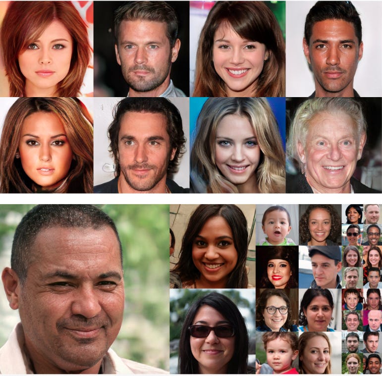
I bet most of us have seen a lot of AI-generated people faces in recent times, be it in papers or blogs. We have reached a stage where it is becoming increasingly difficult to distinguish between actual human faces and faces that are generated by Artificial Intelligence.

In this post, I will help the reader to understand how they can create and build such applications on their own.

I will try to keep this post as intuitive as possible for starters while not dumbing it down too much.

This post is about understanding how GANs work.


Task Overview

I will work on creating our own anime characters using anime characters dataset.

The DC-GAN flavor of GANs which I will use here is widely applicable not only to generate Faces or new anime characters; it can also be used to create modern fashion styles, for general content creation and sometimes for data augmentation purposes as well.

As per my view, GANs will change the way video games and special effects are generated. The approach could create realistic textures or characters on demand.

You can find the full code for this chapter in the Github Repository . I have also uploaded the code to Google Colab so that you can try it yourself.


Using DCGAN architecture to generate anime images

As always before we get into the coding, it helps to delve a little bit into the theory.

The main idea of DC-GAN’s stemmed from the paper UNSUPERVISED REPRESENTATION LEARNING WITH DEEP CONVOLUTIONAL GENERATIVE ADVERSARIAL NETWORKS written in 2016 by Alec Radford, Luke Metz, and Soumith Chintala.

Although I am going to explain the paper in the next few sections, do take a look at it. It is an excellent paper.


INTUITION: Brief Intro to GANs for Generating Fake Images

Generator vs. Discriminator

Typically, GANs employ two dueling neural networks to train a computer to learn the nature of a data set well enough to generate convincing fakes.

We can think of this as two systems where one Neural Network works to generate fakes (Generator), and another neural network (Discriminator) tries to classify which image is a fake.

As both generator and discriminator networks do this repetitively, the networks eventually get better at their respective tasks.

Think of this as simple as swordplay. Two noobs start sparring with each other. After a while, both become better at swordplay.

Or you could think of this as a robber(generator) and a policeman(Discriminator). After a lot of thefts, the robber becomes better at thieving while the policeman gets better at catching the robber. In an ideal world.

The Losses in these neural networks are primarily a function of how the other network performs:

  • Discriminator network loss is a function of generator network quality- Loss is high for the discriminator if it gets fooled by the generator’s fake images

  • Generator network loss is a function of discriminator network quality — Loss is high if the generator is not able to fool the discriminator.

In the training phase, we train our Discriminator and Generator networks sequentially intending to improve both the Discriminator and Generator performance.

The objective is to end up with weights that help Generators to generate realistic looking images. In the end, we can use the Generator Neural network to generate fake images from Random Noise.


Generator architecture

One of the main problems we face with GANs is that the training is not very stable. Thus we have to come up with a Generator architecture that solves our problem and also results in stable training.

The preceding diagram is taken from the paper, which explains the DC-GAN generator architecture. It might look a little bit confusing.

Essentially we can think of a generator Neural Network as a black box which takes as input a 100 sized normally generated vector of numbers and gives us an image:

How do we get such an architecture?

In the below architecture, we use a dense layer of size 4x4x1024 to create a dense vector out of this 100-d vector. Then, we reshape this dense vector in the shape of an image of 4x4 with 1024 filters, as shown in the following figure:

tc

We don’t have to worry about any weights right now as the network itself will learn those while training.

Once we have the 1024 4x4 maps, we do upsampling using a series of Transposed convolutions, which after each operation doubles the size of the image and halves the number of maps. In the last step, though we don’t half the number of maps but reduce it to 3 channels/maps only for each RGB channel since we need three channels for the output image.

Now, What are Transpose convolutions?

In most simple terms, transpose convolutions provide us with a way to upsample images. While in the convolution operation we try to go from a 4x4 image to a 2x2 image, in Transpose convolutions, we convolve from 2x2 to 4x4 as shown in the following figure:

Q: We know that Un-pooling is popularly used for upsampling input feature maps in the convolutional neural network (CNN). Why don’t we use Un-pooling?

It is because un-pooling does not involve any learning. However, transposed convolution is learnable, and that is why we prefer transposed convolutions to un-pooling. Their parameters can be learned by the generator as we will see in some time.

Discriminator architecture

Now, as we have understood the generator architecture, here is the discriminator as a black box.

In practice, it contains a series of convolutional layers and a dense layer at the end to predict if an image is fake or not as shown in the following figure:

Takes an image as input and predicts if it is real/fake. Every image conv net ever.

Data preprocessing and visualization

The first thing we want to do is to look at some of the images in the dataset. The following are the python commands to visualize some of the images from the dataset:

filenames = glob.glob('animeface-character-dataset/*/*.pn*')
plt.figure(figsize=(10, 8))
for i in range(5):
    img = plt.imread(filenames[i], 0)
    plt.subplot(4, 5, i+1)
    plt.imshow(img)
    plt.title(img.shape)
    plt.xticks([])
    plt.yticks([])
plt.tight_layout()
plt.show()

The resultant output is as follows:

We get to see the sizes of the images and the images themselves.

We also need functions to preprocess the images to a standard size of 64x64x3, in this particular case, before proceeding further with our training.

We will also need to normalize the image pixels before we use it to train our GAN. You can see the code it is well commented.

# A function to normalize image pixels.
def norm_img(img):
    '''A function to Normalize Images.
    Input:
        img : Original image as numpy array.
    Output: Normailized Image as numpy array
    '''
    img = (img / 127.5) - 1
    return img
def denorm_img(img):
    '''A function to Denormailze, i.e. recreate image from normalized image
    Input:
        img : Normalized image as numpy array.
    Output: Original Image as numpy array
    '''
    img = (img + 1) * 127.5
    return img.astype(np.uint8)
def sample_from_dataset(batch_size, image_shape, data_dir=None):
    '''Create a batch of image samples by sampling random images from a data directory.
    Resizes the image using image_shape and normalize the images.
    Input:
        batch_size : Sample size required
        image_size : Size that Image should be resized to
        data_dir : Path of directory where training images are placed.
    Output:
        sample : batch of processed images
    '''
    sample_dim = (batch_size,) + image_shape
    sample = np.empty(sample_dim, dtype=np.float32)
    all_data_dirlist = list(glob.glob(data_dir))
    sample_imgs_paths = np.random.choice(all_data_dirlist,batch_size)
    for index,img_filename in enumerate(sample_imgs_paths):
        image = Image.open(img_filename)
        image = image.resize(image_shape[:-1])
        image = image.convert('RGB')
        image = np.asarray(image)
        image = norm_img(image)
        sample[index,...] = image
    return sample

As you will see, we will be using the preceding defined functions in the training part of our code.

Implementation of DCGAN

This is the part where we define our DCGAN. We will be defining our noise generator function, Generator architecture, and Discriminator architecture.

Generating noise vector for Generator

Kids: Normal Noise generators

The following code block is a helper function to create a noise vector of predefined length for a Generator. It will generate the noise which we want to convert to an image using our generator architecture.

We use a normal distribution

MLWhiz: Data Science, Machine Learning, Artificial Intelligence

to generate the noise vector:

def gen_noise(batch_size, noise_shape):
    ''' Generates a numpy vector sampled from normal distribution of shape                                (batch_size,noise_shape)
    Input:
        batch_size : size of batch
        noise_shape: shape of noise vector, normally kept as 100
    Output:a numpy vector sampled from normal distribution of shape                                  (batch_size,noise_shape)     
    '''
    return np.random.normal(0, 1, size=(batch_size,)+noise_shape)

Generator architecture

The Generator is the most crucial part of the GAN.

Here, I create a generator by adding some transposed convolution layers to upsample the noise vector to an image.

As you will notice, this generator architecture is not the same as given in the Original DC-GAN paper.

I needed to make some architectural changes to fit our data better, so I added a convolution layer in the middle and removed all dense layers from the generator architecture, making it fully convolutional.

I also use a lot of Batchnorm layers with a momentum of 0.5 and leaky ReLU activation. I use Adam optimizer with β=0.5. The following code block is the function I will use to create the generator:

def get_gen_normal(noise_shape):
    ''' This function takes as input shape of the noise vector and creates the Keras generator    architecture.
    '''
    kernel_init = 'glorot_uniform'    
    gen_input = Input(shape = noise_shape)

    # Transpose 2D conv layer 1.
    generator = Conv2DTranspose(filters = 512, kernel_size = (4,4), strides = (1,1), padding = "valid", data_format = "channels_last", kernel_initializer = kernel_init)(gen_input)
    generator = BatchNormalization(momentum = 0.5)(generator)
    generator = LeakyReLU(0.2)(generator)

    # Transpose 2D conv layer 2.
    generator = Conv2DTranspose(filters = 256, kernel_size = (4,4), strides = (2,2), padding = "same", data_format = "channels_last", kernel_initializer = kernel_init)(generator)
    generator = BatchNormalization(momentum = 0.5)(generator)
    generator = LeakyReLU(0.2)(generator)

    # Transpose 2D conv layer 3.
    generator = Conv2DTranspose(filters = 128, kernel_size = (4,4), strides = (2,2), padding = "same", data_format = "channels_last", kernel_initializer = kernel_init)(generator)
    generator = BatchNormalization(momentum = 0.5)(generator)
    generator = LeakyReLU(0.2)(generator)

    # Transpose 2D conv layer 4.
    generator = Conv2DTranspose(filters = 64, kernel_size = (4,4), strides = (2,2), padding = "same", data_format = "channels_last", kernel_initializer = kernel_init)(generator)
    generator = BatchNormalization(momentum = 0.5)(generator)
    generator = LeakyReLU(0.2)(generator)

    # conv 2D layer 1.
    generator = Conv2D(filters = 64, kernel_size = (3,3), strides = (1,1), padding = "same", data_format = "channels_last", kernel_initializer = kernel_init)(generator)
    generator = BatchNormalization(momentum = 0.5)(generator)
    generator = LeakyReLU(0.2)(generator)

    # Final Transpose 2D conv layer 5 to generate final image. Filter size 3 for 3 image channel
    generator = Conv2DTranspose(filters = 3, kernel_size = (4,4), strides = (2,2), padding = "same", data_format = "channels_last", kernel_initializer = kernel_init)(generator)

    # Tanh activation to get final normalized image
    generator = Activation('tanh')(generator)

    # defining the optimizer and compiling the generator model.
    gen_opt = Adam(lr=0.00015, beta_1=0.5)
    generator_model = Model(input = gen_input, output = generator)
    generator_model.compile(loss='binary_crossentropy', optimizer=gen_opt, metrics=['accuracy'])
    generator_model.summary()
    return generator_model

You can plot the final generator model:

plot_model(generator, to_file='gen_plot.png', show_shapes=True, show_layer_names=True)
Generator Architecture

Discriminator architecture

Here is the discriminator architecture where I use a series of convolutional layers and a dense layer at the end to predict if an image is fake or not.

Here is the architecture of the discriminator:

def get_disc_normal(image_shape=(64,64,3)):
    dropout_prob = 0.4
    kernel_init = 'glorot_uniform'
    dis_input = Input(shape = image_shape)

    # Conv layer 1:
    discriminator = Conv2D(filters = 64, kernel_size = (4,4), strides = (2,2), padding = "same", data_format = "channels_last", kernel_initializer = kernel_init)(dis_input)
    discriminator = LeakyReLU(0.2)(discriminator)
    # Conv layer 2:
    discriminator = Conv2D(filters = 128, kernel_size = (4,4), strides = (2,2), padding = "same", data_format = "channels_last", kernel_initializer = kernel_init)(discriminator)
    discriminator = BatchNormalization(momentum = 0.5)(discriminator)
    discriminator = LeakyReLU(0.2)(discriminator)
    # Conv layer 3:   
    discriminator = Conv2D(filters = 256, kernel_size = (4,4), strides = (2,2), padding = "same", data_format = "channels_last", kernel_initializer = kernel_init)(discriminator)
    discriminator = BatchNormalization(momentum = 0.5)(discriminator)
    discriminator = LeakyReLU(0.2)(discriminator)
    # Conv layer 4:
    discriminator = Conv2D(filters = 512, kernel_size = (4,4), strides = (2,2), padding = "same", data_format = "channels_last", kernel_initializer = kernel_init)(discriminator)
    discriminator = BatchNormalization(momentum = 0.5)(discriminator)
    discriminator = LeakyReLU(0.2)(discriminator)#discriminator = MaxPooling2D(pool_size=(2, 2))(discriminator)
    # Flatten
    discriminator = Flatten()(discriminator)
    # Dense Layer
    discriminator = Dense(1)(discriminator)
    # Sigmoid Activation
    discriminator = Activation('sigmoid')(discriminator)
    # Optimizer and Compiling model
    dis_opt = Adam(lr=0.0002, beta_1=0.5)
    discriminator_model = Model(input = dis_input, output = discriminator)
    discriminator_model.compile(loss='binary_crossentropy', optimizer=dis_opt, metrics=['accuracy'])
    discriminator_model.summary()
    return discriminator_model
plot_model(discriminator, to_file='dis_plot.png', show_shapes=True, show_layer_names=True)
Discriminator Architecture

Training

MLWhiz: Data Science, Machine Learning, Artificial Intelligence

Understanding how the training works in GAN is essential. And maybe a little interesting too.

I start by creating our discriminator and generator using the functions defined in the previous section:

discriminator = get_disc_normal(image_shape)
generator = get_gen_normal(noise_shape)

The generator and discriminator are then combined to create the final GAN.

discriminator.trainable = False

# Optimizer for the GAN
opt = Adam(lr=0.00015, beta_1=0.5) #same as generator
# Input to the generator
gen_inp = Input(shape=noise_shape)

GAN_inp = generator(gen_inp)
GAN_opt = discriminator(GAN_inp)

# Final GAN
gan = Model(input = gen_inp, output = GAN_opt)
gan.compile(loss = 'binary_crossentropy', optimizer = opt, metrics=['accuracy'])

plot_model(gan, to_file='gan_plot.png', show_shapes=True, show_layer_names=True)

This is the architecture of our whole GAN:

MLWhiz: Data Science, Machine Learning, Artificial Intelligence

The Training Loop

This is the main region where we need to understand how the blocks we have created until now assemble and work together to work as one.

# Use a fixed noise vector to see how the GAN Images transition through time on a fixed noise.
fixed_noise = gen_noise(16,noise_shape)

# To keep Track of losses
avg_disc_fake_loss = []
avg_disc_real_loss = []
avg_GAN_loss = []

# We will run for num_steps iterations
for step in range(num_steps):
    tot_step = step
    print("Begin step: ", tot_step)
    # to keep track of time per step
    step_begin_time = time.time()

    # sample a batch of normalized images from the dataset
    real_data_X = sample_from_dataset(batch_size, image_shape, data_dir=data_dir)

    # Genearate noise to send as input to the generator
    noise = gen_noise(batch_size,noise_shape)

    # Use generator to create(predict) images
    fake_data_X = generator.predict(noise)

    # Save predicted images from the generator every 10th step
    if (tot_step % 100) == 0:
        step_num = str(tot_step).zfill(4)
        save_img_batch(fake_data_X,img_save_dir+step_num+"_image.png")

    # Create the labels for real and fake data. We don't give exact ones and zeros but add a small amount of noise. This is an important GAN training trick
    real_data_Y = np.ones(batch_size) - np.random.random_sample(batch_size)*0.2
    fake_data_Y = np.random.random_sample(batch_size)*0.2

    # train the discriminator using data and labels

    discriminator.trainable = True
    generator.trainable = False

    # Training Discriminator seperately on real data
    dis_metrics_real = discriminator.train_on_batch(real_data_X,real_data_Y)
    # training Discriminator seperately on fake data
    dis_metrics_fake = discriminator.train_on_batch(fake_data_X,fake_data_Y)

    print("Disc: real loss: %f fake loss: %f" % (dis_metrics_real[0], dis_metrics_fake[0]))

    # Save the losses to plot later
    avg_disc_fake_loss.append(dis_metrics_fake[0])
    avg_disc_real_loss.append(dis_metrics_real[0])

    # Train the generator using a random vector of noise and its labels (1's with noise)
    generator.trainable = True
    discriminator.trainable = False

    GAN_X = gen_noise(batch_size,noise_shape)
    GAN_Y = real_data_Y

    gan_metrics = gan.train_on_batch(GAN_X,GAN_Y)
    print("GAN loss: %f" % (gan_metrics[0]))

    # Log results by opening a file in append mode
    text_file = open(log_dir+"\\training_log.txt", "a")
    text_file.write("Step: %d Disc: real loss: %f fake loss: %f GAN loss: %f\n" % (tot_step, dis_metrics_real[0], dis_metrics_fake[0],gan_metrics[0]))
    text_file.close()

    # save GAN loss to plot later
    avg_GAN_loss.append(gan_metrics[0])

    end_time = time.time()
    diff_time = int(end_time - step_begin_time)
    print("Step %d completed. Time took: %s secs." % (tot_step, diff_time))

    # save model at every 500 steps
    if ((tot_step+1) % 500) == 0:
        print("-----------------------------------------------------------------")
        print("Average Disc_fake loss: %f" % (np.mean(avg_disc_fake_loss)))
        print("Average Disc_real loss: %f" % (np.mean(avg_disc_real_loss)))
        print("Average GAN loss: %f" % (np.mean(avg_GAN_loss)))
        print("-----------------------------------------------------------------")
        discriminator.trainable = False
        generator.trainable = False
        # predict on fixed_noise
        fixed_noise_generate = generator.predict(noise)
        step_num = str(tot_step).zfill(4)
        save_img_batch(fixed_noise_generate,img_save_dir+step_num+"fixed_image.png")
        generator.save(save_model_dir+str(tot_step)+"_GENERATOR_weights_and_arch.hdf5")
        discriminator.save(save_model_dir+str(tot_step)+"_DISCRIMINATOR_weights_and_arch.hdf5")

Don’t worry, I will try to break the above code step by step here. The main steps in every training iteration are:

Step 1: Sample a batch of normalized images from the dataset directory

# Use a fixed noise vector to see how the GAN Images transition through time on a fixed noise.
fixed_noise = gen_noise(16,noise_shape)

# To keep Track of losses
avg_disc_fake_loss = []
avg_disc_real_loss = []
avg_GAN_loss = []

# We will run for num_steps iterations
for step in range(num_steps):
    tot_step = step
    print("Begin step: ", tot_step)
    # to keep track of time per step
    step_begin_time = time.time()

    # sample a batch of normalized images from the dataset
    real_data_X = sample_from_dataset(batch_size, image_shape, data_dir=data_dir)

**Step2:**Generate noise for input to the generator

# Generate noise to send as input to the generator
    noise = gen_noise(batch_size,noise_shape)

**Step3:**Generate images using random noise using the generator.

# Use generator to create(predict) images
    fake_data_X = generator.predict(noise)

    # Save predicted images from the generator every 100th step
    if (tot_step % 100) == 0:
        step_num = str(tot_step).zfill(4)

save_img_batch(fake_data_X,img_save_dir+step_num+"_image.png")

**Step 4:**Train discriminator using generator images(Fake images) and real normalized images(Real Images) and their noisy labels.

# Create the labels for real and fake data. We don't give exact ones and zeros but add a small amount of noise. This is an important GAN training trick
    real_data_Y = np.ones(batch_size) - np.random.random_sample(batch_size)*0.2
    fake_data_Y = np.random.random_sample(batch_size)*0.2

    # train the discriminator using data and labels

discriminator.trainable = True
    generator.trainable = False

# Training Discriminator seperately on real data
    dis_metrics_real = discriminator.train_on_batch(real_data_X,real_data_Y)
    # training Discriminator seperately on fake data
    dis_metrics_fake = discriminator.train_on_batch(fake_data_X,fake_data_Y)

    print("Disc: real loss: %f fake loss: %f" % (dis_metrics_real[0], dis_metrics_fake[0]))

    # Save the losses to plot later
    avg_disc_fake_loss.append(dis_metrics_fake[0])
    avg_disc_real_loss.append(dis_metrics_real[0])

**Step 5:**Train the GAN using noise as X and 1’s(noisy) as Y while keeping discriminator as untrainable.

# Train the generator using a random vector of noise and its labels (1's with noise)
    generator.trainable = True
    discriminator.trainable = False

GAN_X = gen_noise(batch_size,noise_shape)
    GAN_Y = real_data_Y

    gan_metrics = gan.train_on_batch(GAN_X,GAN_Y)
    print("GAN loss: %f" % (gan_metrics[0]))

We repeat the steps using the for loop to end up with a good discriminator and generator.

Results

The final output image looks like the following. As we can see, the GAN can generate pretty good images for our content editor friends to work with.

They might be a little crude for your liking, but still, this project was a starter for our GAN journey.

</figure>

Loss over the training period

Here is the graph generated for the losses. We can see that the GAN Loss is decreasing on average and the variance is decreasing too as we do more steps. One might want to train for even more iterations to get better results.

MLWhiz: Data Science, Machine Learning, Artificial Intelligence

Image generated at every 1500 steps

You can see the output and running code in Colab :

# Generating GIF from PNGs
import imageio
# create a list of PNGs
generated_images = [img_save_dir+str(x).zfill(4)+"_image.png" for x in range(0,num_steps,100)]
images = []
for filename in generated_images:
    images.append(imageio.imread(filename))
imageio.mimsave(img_save_dir+'movie.gif', images)
from IPython.display import Image
with open(img_save_dir+'movie.gif','rb') as f:
    display(Image(data=f.read(), format='png'))

MLWhiz: Data Science, Machine Learning, Artificial Intelligence

Given below is the code to generate some images at different training steps. As we can see, as the number of steps increases the images are getting better.

# create a list of 20 PNGs to show
generated_images = [img_save_dir+str(x).zfill(4)+"fixed_image.png" for x in range(0,num_steps,1500)]
print("Displaying generated images")
# You might need to change grid size and figure size here according to num images.
plt.figure(figsize=(16,20))
gs1 = gridspec.GridSpec(5, 4)
gs1.update(wspace=0, hspace=0)
for i,image in enumerate(generated_images):
    ax1 = plt.subplot(gs1[i])
    ax1.set_aspect('equal')
    step = image.split("fixed")[0]
    image = Image.open(image)
    fig = plt.imshow(image)
    # you might need to change some params here
    fig = plt.text(20,47,"Step: "+step,bbox=dict(facecolor='red', alpha=0.5),fontsize=12)
    plt.axis('off')
    fig.axes.get_xaxis().set_visible(False)
    fig.axes.get_yaxis().set_visible(False)
plt.tight_layout()
plt.savefig("GENERATEDimage.png",bbox_inches='tight',pad_inches=0)
plt.show()

Given below is the result of the GAN at different time steps:

MLWhiz: Data Science, Machine Learning, Artificial Intelligence

Conclusion

In this post, we learned about the basics of GAN. We also learned about the Generator and Discriminator architecture for DC-GANs, and we built a simple DC-GAN to generate anime images from scratch.

This model is not very good at generating fake images, yet we get to understand the basics of GANs with this project, and we are fired up to build more exciting and complex GANs as we go forward.

The DC-GAN flavor of GANs is widely applicable not only to generate Faces or new anime characters, but it can also be used to generate new fashion styles, for general content creation and sometimes for data augmentation purposes as well.

We can now conjure up realistic textures or characters on demand if we have the training data at hand, and that is no small feat.

If you want to know more about deep learning applications and use cases, take a look at the Sequence Models course in the Deep Learning Specialization by Andrew NG. Andrew is a great instructor, and this course is great too.

I am going to be writing more of such posts in the future too. Let me know what you think about the series. Follow me up at <strong>Medium</strong> or Subscribe to my <strong>blog</strong> .

Start your future with a Data Analysis Certificate.
comments powered by Disqus