Using XGBoost for time series prediction tasks

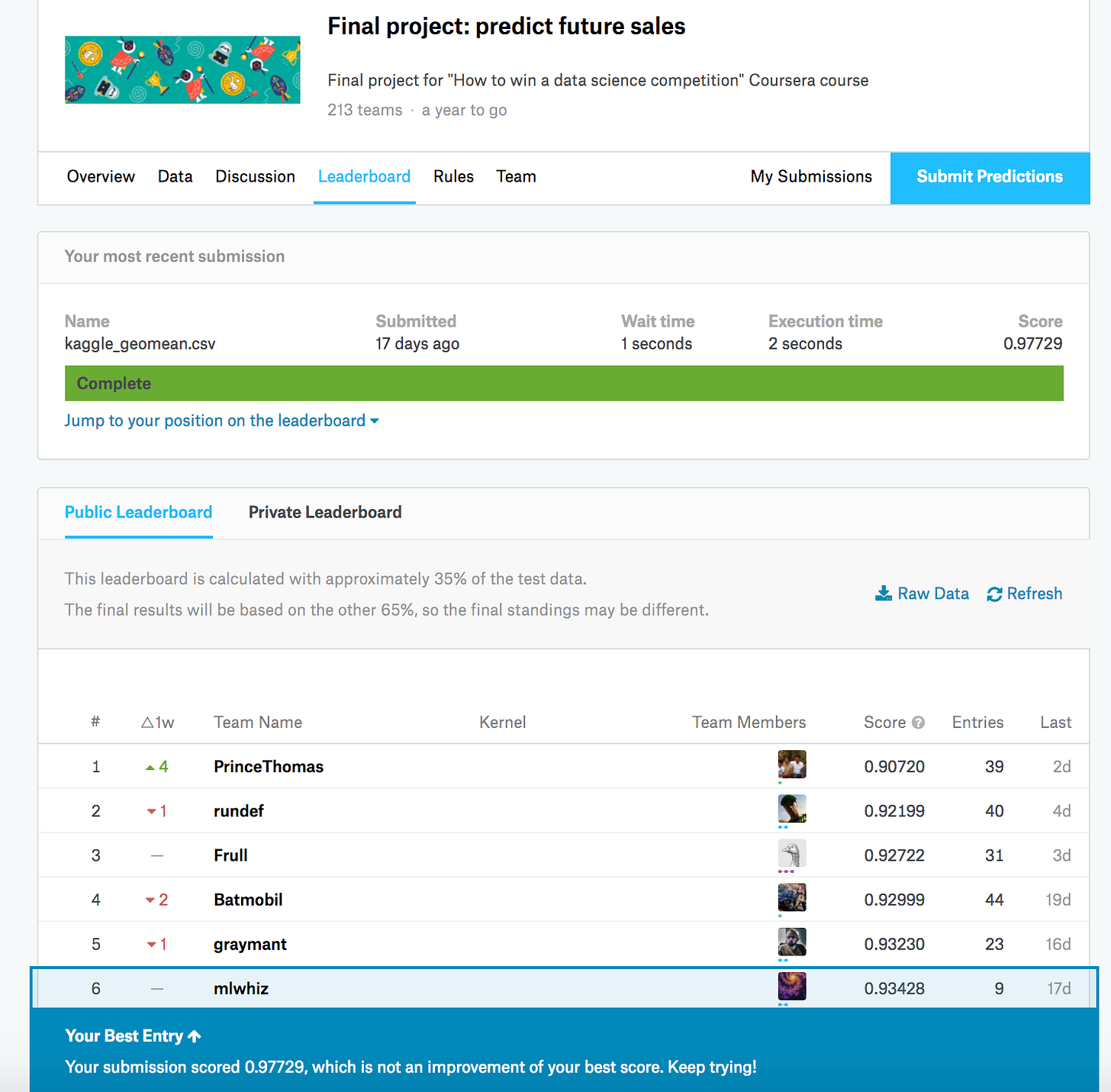
Recently Kaggle master Kazanova along with some of his friends released a “How to win a data science competition” Coursera course. You can start for free with the 7-day Free Trial. The Course involved a final project which itself was a time series prediction problem. Here I will describe how I got a top 10 position as of writing this article.

Description of the Problem:

In this competition we were given a challenging time-series dataset consisting of daily sales data, kindly provided by one of the largest Russian software firms - 1C Company.

We were asked you to predict total sales for every product and store in the next month.

The evaluation metric was RMSE where True target values are clipped into [0,20] range. This target range will be a lot important in understanding the submissions that I will prepare.

The main thing that I noticed was that the data preparation aspect of this competition was by far the most important thing. I creted a variety of features. Here are the steps I took and the features I created.

1. Created a dataframe of all Date_block_num, Store and Item combinations:

This is important because in the months we don’t have a data for an item store combination, the machine learning algorithm needs to be specifically told that the sales is zero.

from itertools import product
# Create "grid" with columns
index_cols = ['shop_id', 'item_id', 'date_block_num']

# For every month we create a grid from all shops/items combinations from that month
grid = []
for block_num in sales['date_block_num'].unique():
    cur_shops = sales.loc[sales['date_block_num'] == block_num, 'shop_id'].unique()
    cur_items = sales.loc[sales['date_block_num'] == block_num, 'item_id'].unique()
    grid.append(np.array(list(product(*[cur_shops, cur_items, [block_num]])),dtype='int32'))
grid = pd.DataFrame(np.vstack(grid), columns = index_cols,dtype=np.int32)

2. Cleaned up a little of sales data after some basic EDA:

sales = sales[sales.item_price<100000]
sales = sales[sales.item_cnt_day<=1000]

3. Created Mean Encodings:

sales_m = sales.groupby(['date_block_num','shop_id','item_id']).agg({'item_cnt_day': 'sum','item_price': np.mean}).reset_index()
sales_m = pd.merge(grid,sales_m,on=['date_block_num','shop_id','item_id'],how='left').fillna(0)
# adding the category id too
sales_m = pd.merge(sales_m,items,on=['item_id'],how='left')

for type_id in ['item_id','shop_id','item_category_id']:
    for column_id,aggregator,aggtype in [('item_price',np.mean,'avg'),('item_cnt_day',np.sum,'sum'),('item_cnt_day',np.mean,'avg')]:

        mean_df = sales.groupby([type_id,'date_block_num']).aggregate(aggregator).reset_index()[[column_id,type_id,'date_block_num']]
        mean_df.columns = [type_id+'_'+aggtype+'_'+column_id,type_id,'date_block_num']

        sales_m = pd.merge(sales_m,mean_df,on=['date_block_num',type_id],how='left')

These above lines add the following 9 features :

• ‘item_id_avg_item_price’

• ‘item_id_sum_item_cnt_day’

• ‘item_id_avg_item_cnt_day’

• ‘shop_id_avg_item_price’,

• ‘shop_id_sum_item_cnt_day’

• ‘shop_id_avg_item_cnt_day’

• ‘item_category_id_avg_item_price’

• ‘item_category_id_sum_item_cnt_day’

• ‘item_category_id_avg_item_cnt_day’

4. Create Lag Features:

Next we create lag features with diferent lag periods on the following features:

• ‘item_id_avg_item_price’,

• ‘item_id_sum_item_cnt_day’

• ‘item_id_avg_item_cnt_day’

• ‘shop_id_avg_item_price’

• ‘shop_id_sum_item_cnt_day’

• ‘shop_id_avg_item_cnt_day’

• ‘item_category_id_avg_item_price’

• ‘item_category_id_sum_item_cnt_day’

• ‘item_category_id_avg_item_cnt_day’

• ‘item_cnt_day’

lag_variables  = list(sales_m.columns[7:])+['item_cnt_day']
lags = [1 ,2 ,3 ,4, 5, 12]
for lag in lags:
    sales_new_df = sales_m.copy()
    sales_new_df.date_block_num+=lag
    sales_new_df = sales_new_df[['date_block_num','shop_id','item_id']+lag_variables]
    sales_new_df.columns = ['date_block_num','shop_id','item_id']+ [lag_feat+'_lag_'+str(lag) for lag_feat in lag_variables]
    sales_means = pd.merge(sales_means, sales_new_df,on=['date_block_num','shop_id','item_id'] ,how='left')

5. Fill NA with zeros:

for feat in sales_means.columns:
    if 'item_cnt' in feat:
        sales_means[feat]=sales_means[feat].fillna(0)
    elif 'item_price' in feat:
        sales_means[feat]=sales_means[feat].fillna(sales_means[feat].median())

6. Drop the columns that we are not going to use in training:

cols_to_drop = lag_variables[:-1] + ['item_name','item_price']

7. Take a recent bit of data only:

sales_means = sales_means[sales_means['date_block_num']>12]

8. Split in train and CV :

X_train = sales_means[sales_means['date_block_num']<33].drop(cols_to_drop, axis=1)
X_cv =  sales_means[sales_means['date_block_num']==33].drop(cols_to_drop, axis=1)

9. THE MAGIC SAUCE:

In the start I told that the clipping aspect of [0,20] will be important. In the next few lines I clipped the days to range[0,40]. You might ask me why 40. An intuitive answer is if I had clipped to range [0,20] there would be very few tree nodes that could give 20 as an answer. While if I increase it to 40 having a 20 becomes much more easier. Please note that We will clip our predictions in the [0,20] range in the end.

def clip(x):
    if x>40:
        return 40
    elif x<0:
        return 0
    else:
        return x
train['item_cnt_day'] = train.apply(lambda x: clip(x['item_cnt_day']),axis=1)
cv['item_cnt_day'] = cv.apply(lambda x: clip(x['item_cnt_day']),axis=1)

10: Modelling:

• Created a XGBoost model to get the most important features(Top 42 features)

• Use hyperopt to tune xgboost

• Used top 10 models from tuned XGBoosts to generate predictions.

• clipped the predictions to [0,20] range

• Final solution was the average of these 10 predictions.

Learned a lot of new things from this awesome course . Most recommended.