The Hitchhikers guide to handle Big Data using Spark

Big Data has become synonymous with Data engineering.

But the line between Data Engineering and Data scientists is blurring day by day.

At this point in time, I think that Big Data must be in the repertoire of all data scientists.

Reason: Too much data is getting generated day by day

And that brings us to Spark.

Now most of the Spark documentation, while good, did not explain it from the perspective of a data scientist.

So I thought of giving it a shot.

This post is going to be about — “How to make Spark work?”

This post is going to be quite long. Actually my longest post on medium, so go pick up a Coffee.

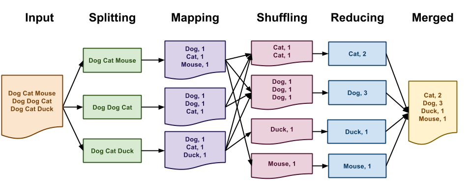
How it all started?-MapReduce

Suppose you are tasked with cutting all the trees in the forest. Perhaps not a good business with all the global warming, but here it serves our purpose and we are talking hypothetically, so I will continue. You have two options:

• Get Batista with an electric powered chainsaw to do your work and make him cut each tree one by one.

• Get 500 normal guys with normal axes and make them work on different trees.

Which would you prefer?

Although Option 1 is still the way some people would go, the need for option 2 led to the emergence of MapReduce.

In Bigdata speak, we call the Batista solution as scaling vertically/scaling-upas in we add/stuff a lot of RAM and hard disk in a single worker.

And the second solution is called scaling horizontally/scaling-sideways. As in you connect a lot of ordinary machines(with less RAM) together and use them in parallel.

Now, vertical scaling has certain benefits over Horizontal scaling:

• It is fast if the size of the problem is small: Think 2 trees. Batista would be through with both of them with his awesome chainsaw while our two guys would be still hacking with their axes.

• It is easy to understand. This is how we have always done things. We normally think about things in a sequential pattern and that is how our whole computer architecture and design has evolved.

But, Horizontal Scaling is

• Less Expensive: Getting 50 normal guys itself is much cheaper than getting a single guy like Batista. Apart from that Batista needs a lot of care and maintenance to keep him cool and he is very sensitive to even small things just like machines with a high amount of RAM.

• Faster when the size of the problem is big: Now imagine 1000 trees and 1000 workers vs a single Batista. With Horizontal Scaling, if we face a very large problem we will just hire 100 or maybe 1000 more cheap workers. It doesn’t work like that with Batista. You have to increase RAM and that means more cooling infrastructure and more maintenance costs.

MapReduce is what makes the second option possible by letting us use a cluster of computers for parallelization.

Now, MapReduce looks like a fairly technical term. But let us break it a little. MapReduce is made up of two terms:

Map:

It is basically the apply/map function. We split our data into n chunks and send each chunk to a different worker(Mapper). If there is any function we would like to apply over the rows of Data our worker does that.

Reduce:

Aggregate the data using some function based on a groupby key. It is basically a groupby.

Of course, there is a lot going in the background to make the system work as intended.

Don’t worry, if you don’t understand it yet. Just keep reading. Maybe you will understand it when we use MapReduce ourselves in the examples I am going to provide.

Why Spark?

Hadoop was the first open source system that introduced us to the MapReduce paradigm of programming and Spark is the system that made it faster, much much faster(100x).

There used to be a lot of data movement in Hadoop as it used to write intermediate results to the file system.

This affected the speed at which you could do analysis.

Spark provided us with an in-memory model, so Spark doesn’t write too much to the disk while working.

Simply, Spark is faster than Hadoop and a lot of people use Spark now.

So without further ado let us get started.

Getting Started with Spark

Installing Spark is actually a headache of its own.

Since we want to understand how it works and really work with it, I would suggest that you use Sparks on Databricks here online with the community edition. Don’t worry it is free.

Once you register and login will be presented with the following screen.

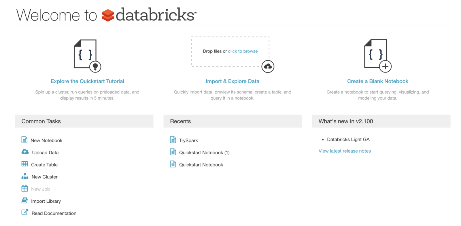
You can start a new notebook here.

Select the Python notebook and give any name to your notebook.

Once you start a new notebook and try to execute any command, the notebook will ask you if you want to start a new cluster. Do it.

The next step will be to check if the sparkcontext is present. To check if the sparkcontext is present you just have to run this command:

sc

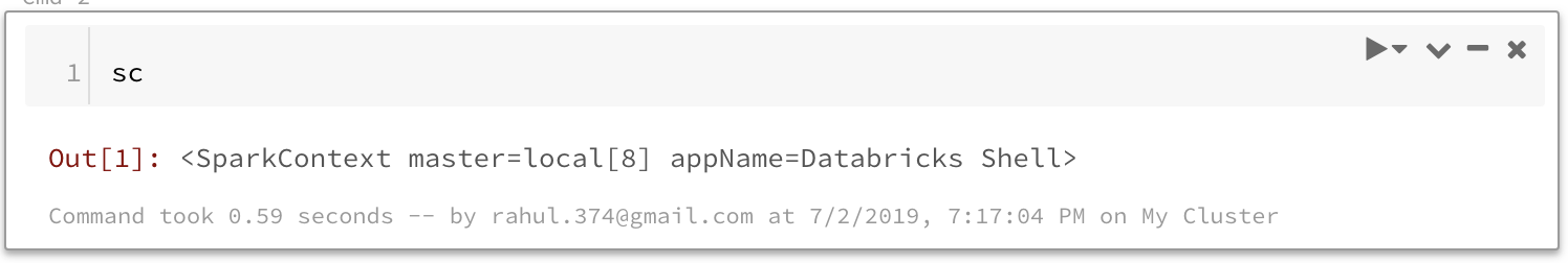
This means that we are set up with a notebook where we can run Spark.

Load Some Data

The next step is to upload some data we will use to learn Spark. Just click on ‘Import and Explore Data’ on the home tab.

I will end up using multiple datasets by the end of this post but let us start with something very simple.

Let us add the file shakespeare.txt which you can download from here .

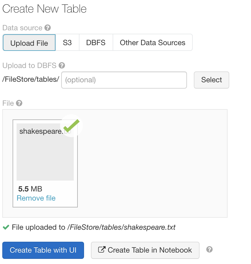
You can see that the file is loaded to /FileStore/tables/shakespeare.txt location.

Our First Spark Program

I like to learn by examples so let’s get done with the “Hello World” of Distributed computing: The WordCount Program.

# Distribute the data - Create a RDD
lines = sc.textFile("/FileStore/tables/shakespeare.txt")

# Create a list with all words, Create tuple (word,1), reduce by key i.e. the word
counts = (lines.flatMap(lambda x: x.split(' '))
                  .map(lambda x: (x, 1))
                  .reduceByKey(lambda x,y : x + y))

# get the output on local
output = counts.take(10)
# print output
for (word, count) in output:
    print("%s: %i" % (word, count))

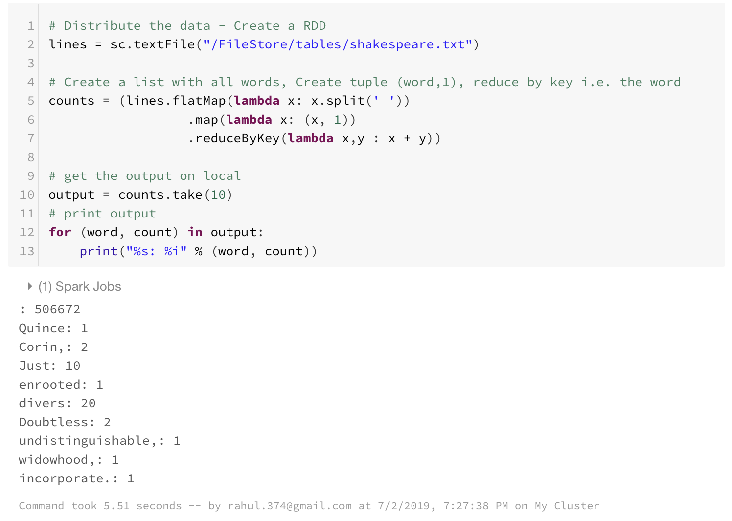
So that is a small example which counts the number of words in the document and prints 10 of them.

And most of the work gets done in the second command.

Don’t worry if you are not able to follow this yet as I still need to tell you about the things that make Spark work.

But before we get into Spark basics, Let us refresh some of our Python Basics. Understanding Spark becomes a lot easier if you have used functional programming with Python.

For those of you who haven’t used it, below is a brief intro.

A functional approach to programming in Python

1. Map

map is used to map a function to an array or a list. Say you want to apply some function to every element in a list.

You can do this by simply using a for loop but python lambda functions let you do this in a single line in Python.

my_list = [1,2,3,4,5,6,7,8,9,10]
# Lets say I want to square each term in my_list.
squared_list = map(lambda x:x**2,my_list)
print(list(squared_list))
------------------------------------------------------------
[1, 4, 9, 16, 25, 36, 49, 64, 81, 100]

In the above example, you could think of map as a function which takes two arguments — A function and a list.

It then applies the function to every element of the list.

What lambda allows you to do is write an inline function. In here the part lambda x:x**2 defines a function that takes x as input and returns x².

You could have also provided a proper function in place of lambda. For example:

def squared(x):
    return x**2

my_list = [1,2,3,4,5,6,7,8,9,10]
# Lets say I want to square each term in my_list.
squared_list = map(squared,my_list)
print(list(squared_list))
------------------------------------------------------------
[1, 4, 9, 16, 25, 36, 49, 64, 81, 100]

The same result, but the lambda expressions make the code compact and a lot more readable.

2. Filter

The other function that is used extensively is the filter function. This function takes two arguments — A condition and the list to filter.

If you want to filter your list using some condition you use filter.

my_list = [1,2,3,4,5,6,7,8,9,10]
# Lets say I want only the even numbers in my list.
filtered_list = filter(lambda x:x%2==0,my_list)
print(list(filtered_list))
---------------------------------------------------------------
[2, 4, 6, 8, 10]

3. Reduce

The next function I want to talk about is the reduce function. This function will be the workhorse in Spark.

This function takes two arguments — a function to reduce that takes two arguments, and a list over which the reduce function is to be applied.

import functools
my_list = [1,2,3,4,5]
# Lets say I want to sum all elements in my list.
sum_list = functools.reduce(lambda x,y:x+y,my_list)
print(sum_list)

In python2 reduce used to be a part of Python, now we have to use reduce as a part of functools.

Here the lambda function takes in two values x, y and returns their sum. Intuitively you can think that the reduce function works as:

    Reduce function first sends 1,2    ; the lambda function returns 3
    Reduce function then sends 3,3     ; the lambda function returns 6
    Reduce function then sends 6,4     ; the lambda function returns 10
    Reduce function finally sends 10,5 ; the lambda function returns 15

A condition on the lambda function we use in reduce is that it must be:

• commutative that is a + b = b + a and

• associative that is (a + b) + c == a + (b + c).

In the above case, we used sum which is commutative as well as associative. Other functions that we could have used: max, min, * etc.

Moving Again to Spark

As we have now got the fundamentals of Python Functional Programming out of the way, lets again head to Spark.

But first, let us delve a little bit into how spark works. Spark actually consists of two things a driver and workers.

Workers normally do all the work and the driver makes them do that work.

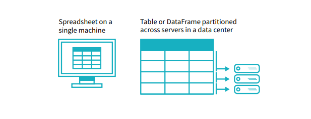
RDD

An RDD(Resilient Distributed Dataset) is a parallelized data structure that gets distributed across the worker nodes. They are the basic units of Spark programming.

In our wordcount example, in the first line

lines = sc.textFile("/FileStore/tables/shakespeare.txt")

We took a text file and distributed it across worker nodes so that they can work on it in parallel. We could also parallelize lists using the function sc.parallelize

For example:

data = [1,2,3,4,5,6,7,8,9,10]
new_rdd = sc.parallelize(data,4)
new_rdd
---------------------------------------------------------------
ParallelCollectionRDD[22] at parallelize at PythonRDD.scala:267

In Spark, we can do two different types of operations on RDD: Transformations and Actions.

1. Transformations: Create new datasets from existing RDDs

2. Actions: Mechanism to get results out of Spark

Transformation Basics

So let us say you have got your data in the form of an RDD.

To requote your data is now accessible to the worker machines. You want to do some transformations on the data now.

You may want to filter, apply some function, etc.

In Spark, this is done using Transformation functions.

Spark provides many transformation functions. You can see a comprehensive list <strong>here</strong> . Some of the main ones that I use frequently are:

1. Map:

Applies a given function to an RDD.

Note that the syntax is a little bit different from Python, but it necessarily does the same thing. Don’t worry about collect yet. For now, just think of it as a function that collects the data in squared_rdd back to a list.

data = [1,2,3,4,5,6,7,8,9,10]
rdd = sc.parallelize(data,4)
squared_rdd = rdd.map(lambda x:x**2)
squared_rdd.collect()
------------------------------------------------------
[1, 4, 9, 16, 25, 36, 49, 64, 81, 100]

2. Filter:

Again no surprises here. Takes as input a condition and keeps only those elements that fulfill that condition.

data = [1,2,3,4,5,6,7,8,9,10]
rdd = sc.parallelize(data,4)
filtered_rdd = rdd.filter(lambda x:x%2==0)
filtered_rdd.collect()
------------------------------------------------------
[2, 4, 6, 8, 10]

3. distinct:

Returns only distinct elements in an RDD.

data = [1,2,2,2,2,3,3,3,3,4,5,6,7,7,7,8,8,8,9,10]
rdd = sc.parallelize(data,4)
distinct_rdd = rdd.distinct()
distinct_rdd.collect()
------------------------------------------------------
[8, 4, 1, 5, 9, 2, 10, 6, 3, 7]

4. flatmap:

Similar to map, but each input item can be mapped to 0 or more output items.

data = [1,2,3,4]
rdd = sc.parallelize(data,4)
flat_rdd = rdd.flatMap(lambda x:[x,x**3])
flat_rdd.collect()
------------------------------------------------------
[1, 1, 2, 8, 3, 27, 4, 64]

5. Reduce By Key:

The parallel to the reduce in Hadoop MapReduce.

Now Spark cannot provide the value if it just worked with Lists.

In Spark, there is a concept of pair RDDs that makes it a lot more flexible. Let’s assume we have a data in which we have a product, its category, and its selling price. We can still parallelize the data.

data = [('Apple','Fruit',200),('Banana','Fruit',24),('Tomato','Fruit',56),('Potato','Vegetable',103),('Carrot','Vegetable',34)]
rdd = sc.parallelize(data,4)

Right now our RDD rdd holds tuples.

Now we want to find out the total sum of revenue that we got from each category.

To do that we have to transform our rdd to a pair rdd so that it only contains key-value pairs/tuples.

category_price_rdd = rdd.map(lambda x: (x[1],x[2]))
category_price_rdd.collect()
-----------------------------------------------------------------
[(‘Fruit’, 200), (‘Fruit’, 24), (‘Fruit’, 56), (‘Vegetable’, 103), (‘Vegetable’, 34)]

Here we used the map function to get it in the format we wanted. When working with textfile, the RDD that gets formed has got a lot of strings. We use map to convert it into a format that we want.

So now our category_price_rdd contains the product category and the price at which the product sold.

Now we want to reduce on the key category and sum the prices. We can do this by:

category_total_price_rdd = category_price_rdd.reduceByKey(lambda x,y:x+y)
category_total_price_rdd.collect()
---------------------------------------------------------
[(‘Vegetable’, 137), (‘Fruit’, 280)]

6. Group By Key:

Similar to reduceByKey but does not reduces just puts all the elements in an iterator. For example, if we wanted to keep as key the category and as the value all the products we would use this function.

Let us again use map to get data in the required form.

data = [('Apple','Fruit',200),('Banana','Fruit',24),('Tomato','Fruit',56),('Potato','Vegetable',103),('Carrot','Vegetable',34)]
rdd = sc.parallelize(data,4)
category_product_rdd = rdd.map(lambda x: (x[1],x[0]))
category_product_rdd.collect()
------------------------------------------------------------
[('Fruit', 'Apple'),  ('Fruit', 'Banana'),  ('Fruit', 'Tomato'),  ('Vegetable', 'Potato'),  ('Vegetable', 'Carrot')]

We then use groupByKey as:

grouped_products_by_category_rdd = category_product_rdd.groupByKey()
findata = grouped_products_by_category_rdd.collect()
for data in findata:
    print(data[0],list(data[1]))
------------------------------------------------------------
Vegetable ['Potato', 'Carrot']
Fruit ['Apple', 'Banana', 'Tomato']

Here the groupByKey function worked and it returned the category and the list of products in that category.

Action Basics

You have filtered your data, mapped some functions on it. Done your computation.

Now you want to get the data on your local machine or save it to a file or show the results in the form of some graphs in excel or any visualization tool.

You will need actions for that. A comprehensive list of actions is provided <strong>here</strong> .

Some of the most common actions that I tend to use are:

1. collect:

We have already used this action many times. It takes the whole RDD and brings it back to the driver program.

2. reduce:

Aggregate the elements of the dataset using a function func (which takes two arguments and returns one). The function should be commutative and associative so that it can be computed correctly in parallel.

rdd = sc.parallelize([1,2,3,4,5])
rdd.reduce(lambda x,y : x+y)
---------------------------------
15

3. take:

Sometimes you will need to see what your RDD contains without getting all the elements in memory itself. take returns a list with the first n elements of the RDD.

rdd = sc.parallelize([1,2,3,4,5])
rdd.take(3)
---------------------------------
[1, 2, 3]

4. takeOrdered:

takeOrdered returns the first n elements of the RDD using either their natural order or a custom comparator.

rdd = sc.parallelize([5,3,12,23])

# descending order
rdd.takeOrdered(3,lambda s:-1*s)
----
[23, 12, 5]

rdd = sc.parallelize([(5,23),(3,34),(12,344),(23,29)])

# descending order
rdd.takeOrdered(3,lambda s:-1*s[1])
---
[(12, 344), (3, 34), (23, 29)]

We have our basics covered finally. Let us get back to our wordcount example

Understanding The WordCount Example

Now we sort of understand the transformations and the actions provided to us by Spark.

It should not be difficult to understand the wordcount program now. Let us go through the program line by line.

The first line creates an RDD and distributes it to the workers.

lines = sc.textFile("/FileStore/tables/shakespeare.txt")

This RDD lines contains a list of sentences in the file. You can see the rdd content using take

lines.take(5)
--------------------------------------------
['The Project Gutenberg EBook of The Complete Works of William Shakespeare, by ',  'William Shakespeare',  '',  'This eBook is for the use of anyone anywhere at no cost and with',  'almost no restrictions whatsoever.  You may copy it, give it away or']

This RDD is of the form:

['word1 word2 word3','word4 word3 word2']

This next line is actually the workhorse function in the whole script.

counts = (lines.flatMap(lambda x: x.split(' '))
                  .map(lambda x: (x, 1))
                  .reduceByKey(lambda x,y : x + y))

It contains a series of transformations that we do to the lines RDD. First of all, we do a flatmap transformation.

The flatmap transformation takes as input the lines and gives words as output. So after the flatmap transformation, the RDD is of the form:

['word1','word2','word3','word4','word3','word2']

Next, we do a map transformation on the flatmap output which converts the RDD to :

[('word1',1),('word2',1),('word3',1),('word4',1),('word3',1),('word2',1)]

Finally, we do a reduceByKey transformation which counts the number of time each word appeared.

After which the RDD approaches the final desirable form.

[('word1',1),('word2',2),('word3',2),('word4',1)]

This next line is an action that takes the first 10 elements of the resulting RDD locally.

output = counts.take(10)

This line just prints the output

for (word, count) in output:
    print("%s: %i" % (word, count))

And that is it for the wordcount program. Hope you understand it now.

So till now, we talked about the Wordcount example and the basic transformations and actions that you could use in Spark. But we don’t do wordcount in real life.

We have to work on bigger problems which are much more complex. Worry not! Whatever we have learned till now will let us do that and more.

Spark in Action with Example

Let us work with a concrete example which takes care of some usual transformations.

We will work on Movielens ml-100k.zip dataset which is a stable benchmark dataset. 100,000 ratings from 1000 users on 1700 movies. Released 4/1998.

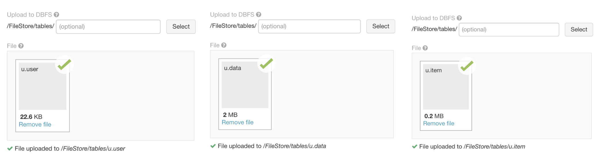
The Movielens dataset contains a lot of files but we are going to be working with 3 files only:

1. Users: This file name is kept as “u.user”, The columns in this file are:

   [‘user_id’, ‘age’, ‘sex’, ‘occupation’, ‘zip_code’]

2. Ratings: This file name is kept as “u.data”, The columns in this file are:

   [‘user_id’, ‘movie_id’, ‘rating’, ‘unix_timestamp’]

3. Movies: This file name is kept as “u.item”, The columns in this file are:

   [‘movie_id’, ‘title’, ‘release_date’, ‘video_release_date’, ‘imdb_url’, and 18 more columns…..]

Let us start by importing these 3 files into our spark instance using ‘Import and Explore Data’ on the home tab.

Our business partner now comes to us and asks us to find out the 25 most rated movie titles from this data. How many times a movie has been rated?

Let us load the data in different RDDs and see what the data contains.

userRDD = sc.textFile("/FileStore/tables/u.user")
ratingRDD = sc.textFile("/FileStore/tables/u.data")
movieRDD = sc.textFile("/FileStore/tables/u.item")
print("userRDD:",userRDD.take(1))
print("ratingRDD:",ratingRDD.take(1))
print("movieRDD:",movieRDD.take(1))
-----------------------------------------------------------
userRDD: ['1|24|M|technician|85711']
ratingRDD: ['196\t242\t3\t881250949']
movieRDD: ['1|Toy Story (1995)|01-Jan-1995||http://us.imdb.com/M/title-exact?Toy%20Story%20(1995)|0|0|0|1|1|1|0|0|0|0|0|0|0|0|0|0|0|0|0']

We note that to answer this question we will need to use the ratingRDD. But the ratingRDD does not have the movie name.

So we would have to merge movieRDD and ratingRDD using movie_id.

How we would do that in Spark?

Below is the code. We also use a new transformation leftOuterJoin. Do read the docs and comments in the below code.

# Create a RDD from RatingRDD that only contains the two columns of interest i.e. movie_id,rating.
RDD_movid_rating = ratingRDD.map(lambda x : (x.split("\t")[1],x.split("\t")[2]))
print("RDD_movid_rating:",RDD_movid_rating.take(4))

# Create a RDD from MovieRDD that only contains the two columns of interest i.e. movie_id,title.
RDD_movid_title = movieRDD.map(lambda x : (x.split("|")[0],x.split("|")[1]))
print("RDD_movid_title:",RDD_movid_title.take(2))

# merge these two pair RDDs based on movie_id. For this we will use the transformation leftOuterJoin(). See the transformation document.
rdd_movid_title_rating = RDD_movid_rating.leftOuterJoin(RDD_movid_title)
print("rdd_movid_title_rating:",rdd_movid_title_rating.take(1))

# use the RDD in previous step to create (movie,1) tuple pair RDD
rdd_title_rating = rdd_movid_title_rating.map(lambda x: (x[1][1],1 ))
print("rdd_title_rating:",rdd_title_rating.take(2))

# Use the reduceByKey transformation to reduce on the basis of movie_title
rdd_title_ratingcnt = rdd_title_rating.reduceByKey(lambda x,y: x+y)
print("rdd_title_ratingcnt:",rdd_title_ratingcnt.take(2))

# Get the final answer by using takeOrdered Transformation
print "#####################################"
print "25 most rated movies:",rdd_title_ratingcnt.takeOrdered(25,lambda x:-x[1])
print "#####################################"

OUTPUT:
--------------------------------------------------------------------RDD_movid_rating: [('242', '3'), ('302', '3'), ('377', '1'), ('51', '2')]
RDD_movid_title: [('1', 'Toy Story (1995)'), ('2', 'GoldenEye (1995)')]
rdd_movid_title_rating: [('1440', ('3', 'Above the Rim (1994)'))] rdd_title_rating: [('Above the Rim (1994)', 1), ('Above the Rim (1994)', 1)]
rdd_title_ratingcnt: [('Mallrats (1995)', 54), ('Michael Collins (1996)', 92)]

#####################################
25 most rated movies: [('Star Wars (1977)', 583), ('Contact (1997)', 509), ('Fargo (1996)', 508), ('Return of the Jedi (1983)', 507), ('Liar Liar (1997)', 485), ('English Patient, The (1996)', 481), ('Scream (1996)', 478), ('Toy Story (1995)', 452), ('Air Force One (1997)', 431), ('Independence Day (ID4) (1996)', 429), ('Raiders of the Lost Ark (1981)', 420), ('Godfather, The (1972)', 413), ('Pulp Fiction (1994)', 394), ('Twelve Monkeys (1995)', 392), ('Silence of the Lambs, The (1991)', 390), ('Jerry Maguire (1996)', 384), ('Chasing Amy (1997)', 379), ('Rock, The (1996)', 378), ('Empire Strikes Back, The (1980)', 367), ('Star Trek: First Contact (1996)', 365), ('Back to the Future (1985)', 350), ('Titanic (1997)', 350), ('Mission: Impossible (1996)', 344), ('Fugitive, The (1993)', 336), ('Indiana Jones and the Last Crusade (1989)', 331)] #####################################

Star Wars is the most rated movie in the Movielens Dataset.

Now we could have done all this in a single command using the below command but the code is a little messy now.

I did this to show that you can use chaining functions with Spark and you could bypass the process of variable creation.

print(((ratingRDD.map(lambda x : (x.split("\t")[1],x.split("\t")[2]))).
     leftOuterJoin(movieRDD.map(lambda x : (x.split("|")[0],x.split("|")[1])))).
     map(lambda x: (x[1][1],1)).
     reduceByKey(lambda x,y: x+y).
     takeOrdered(25,lambda x:-x[1]))

Let us do one more. For practice:

Now we want to find the most highly rated 25 movies using the same dataset. We actually want only those movies which have been rated at least 100 times.

# We already have the RDD rdd_movid_title_rating: [(u'429', (u'5', u'Day the Earth Stood Still, The (1951)'))]
# We create an RDD that contains sum of all the ratings for a particular movie
rdd_title_ratingsum = (rdd_movid_title_rating.
                        map(lambda x: (x[1][1],int(x[1][0]))).
                        reduceByKey(lambda x,y:x+y))

print("rdd_title_ratingsum:",rdd_title_ratingsum.take(2))
# Merge this data with the RDD rdd_title_ratingcnt we created in the last step
# And use Map function to divide ratingsum by rating count.
rdd_title_ratingmean_rating_count = (rdd_title_ratingsum.
                                    leftOuterJoin(rdd_title_ratingcnt).
                                    map(lambda x:(x[0],(float(x[1][0])/x[1][1],x[1][1]))))

print("rdd_title_ratingmean_rating_count:",rdd_title_ratingmean_rating_count.take(1))
# We could use take ordered here only but we want to only get the movies which have count
# of ratings more than or equal to 100 so lets filter the data RDD.
rdd_title_rating_rating_count_gt_100 = (rdd_title_ratingmean_rating_count.
                                        filter(lambda x: x[1][1]>=100))

print("rdd_title_rating_rating_count_gt_100:",rdd_title_rating_rating_count_gt_100.take(1))
# Get the final answer by using takeOrdered Transformation
print("#####################################")
print ("25 highly rated movies:")
print(rdd_title_rating_rating_count_gt_100.takeOrdered(25,lambda x:-x[1][0]))
print("#####################################")

OUTPUT:
------------------------------------------------------------
rdd_title_ratingsum: [('Mallrats (1995)', 186), ('Michael Collins (1996)', 318)]
rdd_title_ratingmean_rating_count: [('Mallrats (1995)', (3.4444444444444446, 54))]
rdd_title_rating_rating_count_gt_100: [('Butch Cassidy and the Sundance Kid (1969)', (3.949074074074074, 216))]

#####################################
25 highly rated movies: [('Close Shave, A (1995)', (4.491071428571429, 112)), ("Schindler's List (1993)", (4.466442953020135, 298)), ('Wrong Trousers, The (1993)', (4.466101694915254, 118)), ('Casablanca (1942)', (4.45679012345679, 243)), ('Shawshank Redemption, The (1994)', (4.445229681978798, 283)), ('Rear Window (1954)', (4.3875598086124405, 209)), ('Usual Suspects, The (1995)', (4.385767790262173, 267)), ('Star Wars (1977)', (4.3584905660377355, 583)), ('12 Angry Men (1957)', (4.344, 125)), ('Citizen Kane (1941)', (4.292929292929293, 198)), ('To Kill a Mockingbird (1962)', (4.292237442922374, 219)), ("One Flew Over the Cuckoo's Nest (1975)", (4.291666666666667, 264)), ('Silence of the Lambs, The (1991)', (4.28974358974359, 390)), ('North by Northwest (1959)', (4.284916201117318, 179)), ('Godfather, The (1972)', (4.283292978208232, 413)), ('Secrets & Lies (1996)', (4.265432098765432, 162)), ('Good Will Hunting (1997)', (4.262626262626263, 198)), ('Manchurian Candidate, The (1962)', (4.259541984732825, 131)), ('Dr. Strangelove or: How I Learned to Stop Worrying and Love the Bomb (1963)', (4.252577319587629, 194)), ('Raiders of the Lost Ark (1981)', (4.252380952380952, 420)), ('Vertigo (1958)', (4.251396648044692, 179)), ('Titanic (1997)', (4.2457142857142856, 350)), ('Lawrence of Arabia (1962)', (4.23121387283237, 173)), ('Maltese Falcon, The (1941)', (4.2101449275362315, 138)), ('Empire Strikes Back, The (1980)', (4.204359673024523, 367))]
#####################################

We have talked about RDDs till now as they are very powerful.

You can use RDDs to work with non-relational databases too.

They let you do a lot of things that you couldn’t do with SparkSQL?

Yes, you can use SQL with Spark too which I am going to talk about now.

Spark DataFrames

Spark has provided DataFrame API for us Data Scientists to work with relational data. Here is the documentation for the adventurous folks.

Remember that in the background it still is all RDDs and that is why the starting part of this post focussed on RDDs.

I will start with some common functionalities you will need to work with Spark DataFrames. Would look a lot like Pandas with some syntax changes.

1. Reading the File

ratings = spark.read.load("/FileStore/tables/u.data",format="csv", sep="\t", inferSchema="true", header="false")

2. Show File

We have two ways to show files using Spark Dataframes.

ratings.show()

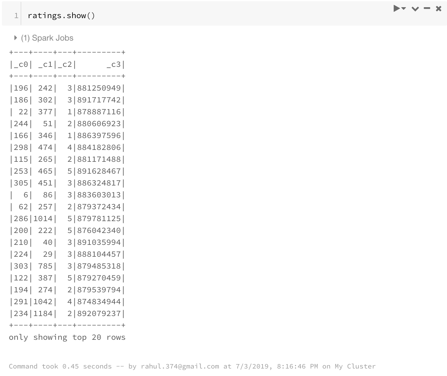
display(ratings)

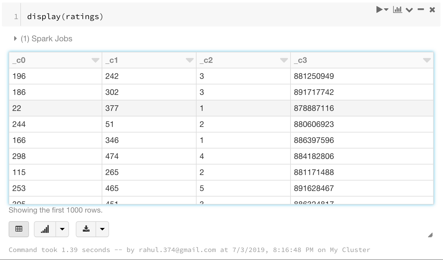
I prefer display as it looks a lot nicer and clean.

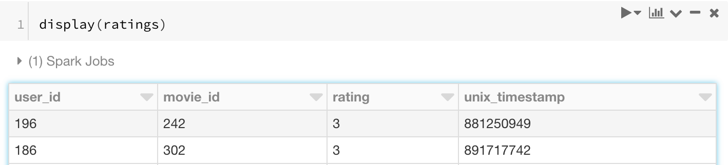
3. Change Column names

Good functionality. Always required. Don’t forget the * in front of the list.

ratings = ratings.toDF(*['user_id', 'movie_id', 'rating', 'unix_timestamp'])
display(ratings)

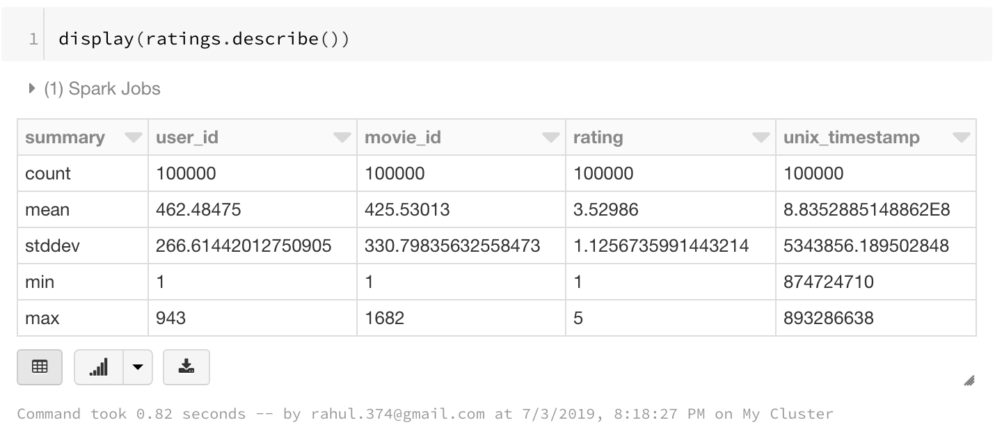
4. Some Basic Stats

print(ratings.count()) #Row Count
print(len(ratings.columns)) #Column Count
---------------------------------------------------------
100000
4

We can also see the dataframe statistics using:

display(ratings.describe())

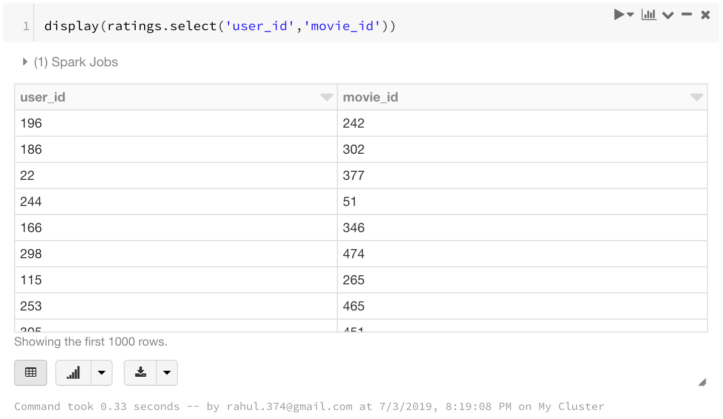
5. Select a few columns

display(ratings.select('user_id','movie_id'))

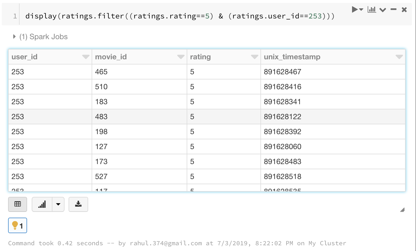
6. Filter

Filter a dataframe using multiple conditions:

display(ratings.filter((ratings.rating==5) & (ratings.user_id==253)))

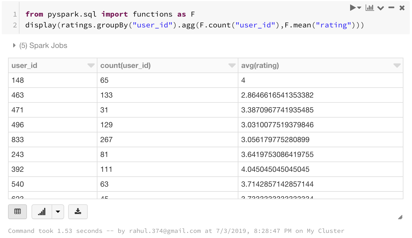
7. Groupby

We can use groupby function with a spark dataframe too. Pretty much same as a pandas groupby with the exception that you will need to import pyspark.sql.functions

from pyspark.sql import functions as F
display(ratings.groupBy("user_id").agg(F.count("user_id"),F.mean("rating")))

Here we have found the count of ratings and average rating from each user_id

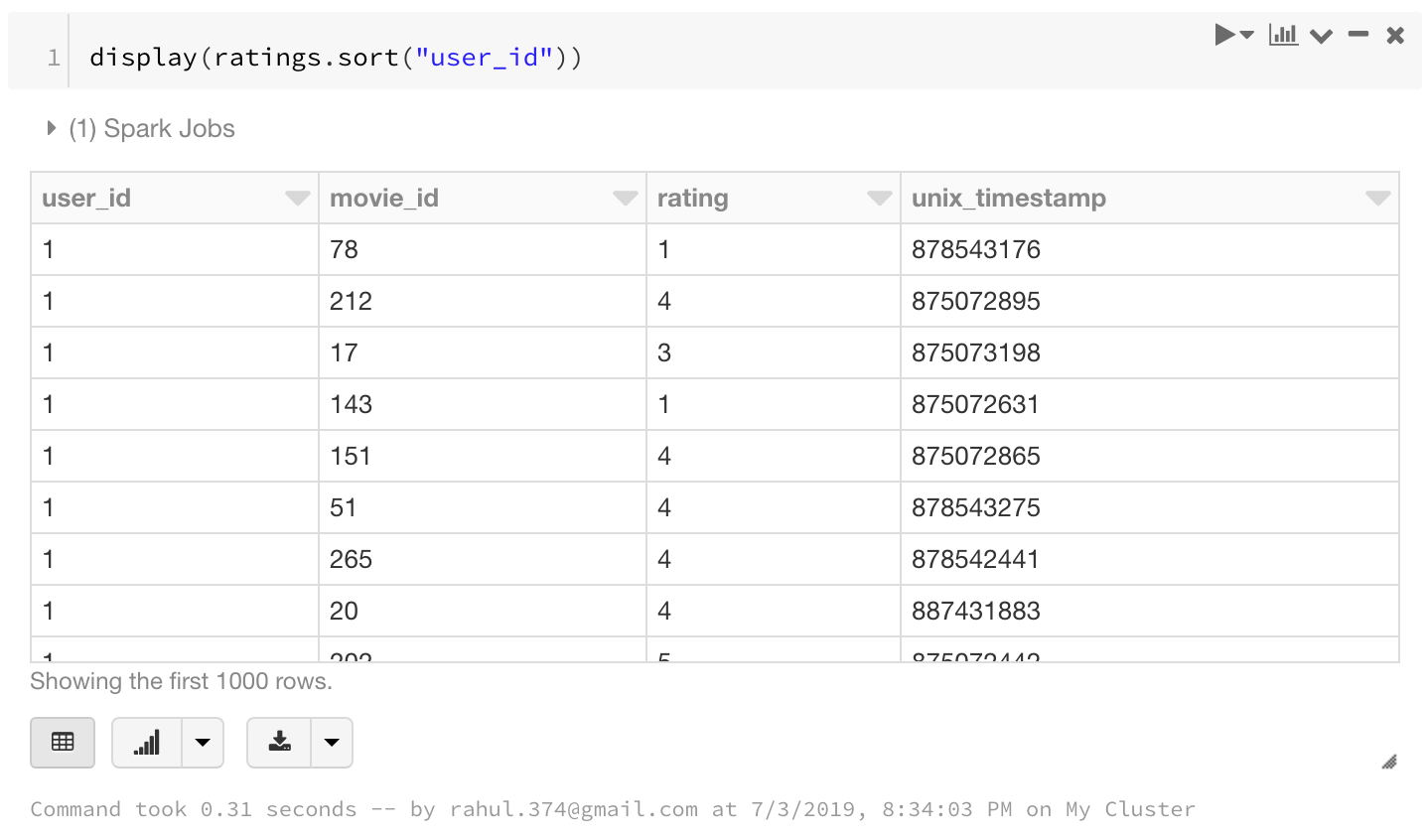
8. Sort

display(ratings.sort("user_id"))

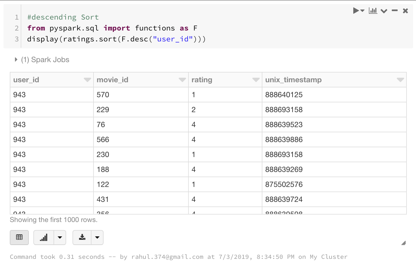
We can also do a descending sort using F.desc function as below.

# descending Sort
from pyspark.sql import functions as F
display(ratings.sort(F.desc("user_id")))

Joins/Merging with Spark Dataframes

I was not able to find a pandas equivalent of merge with Spark DataFrames but we can use SQL with dataframes and thus we can merge dataframes using SQL.

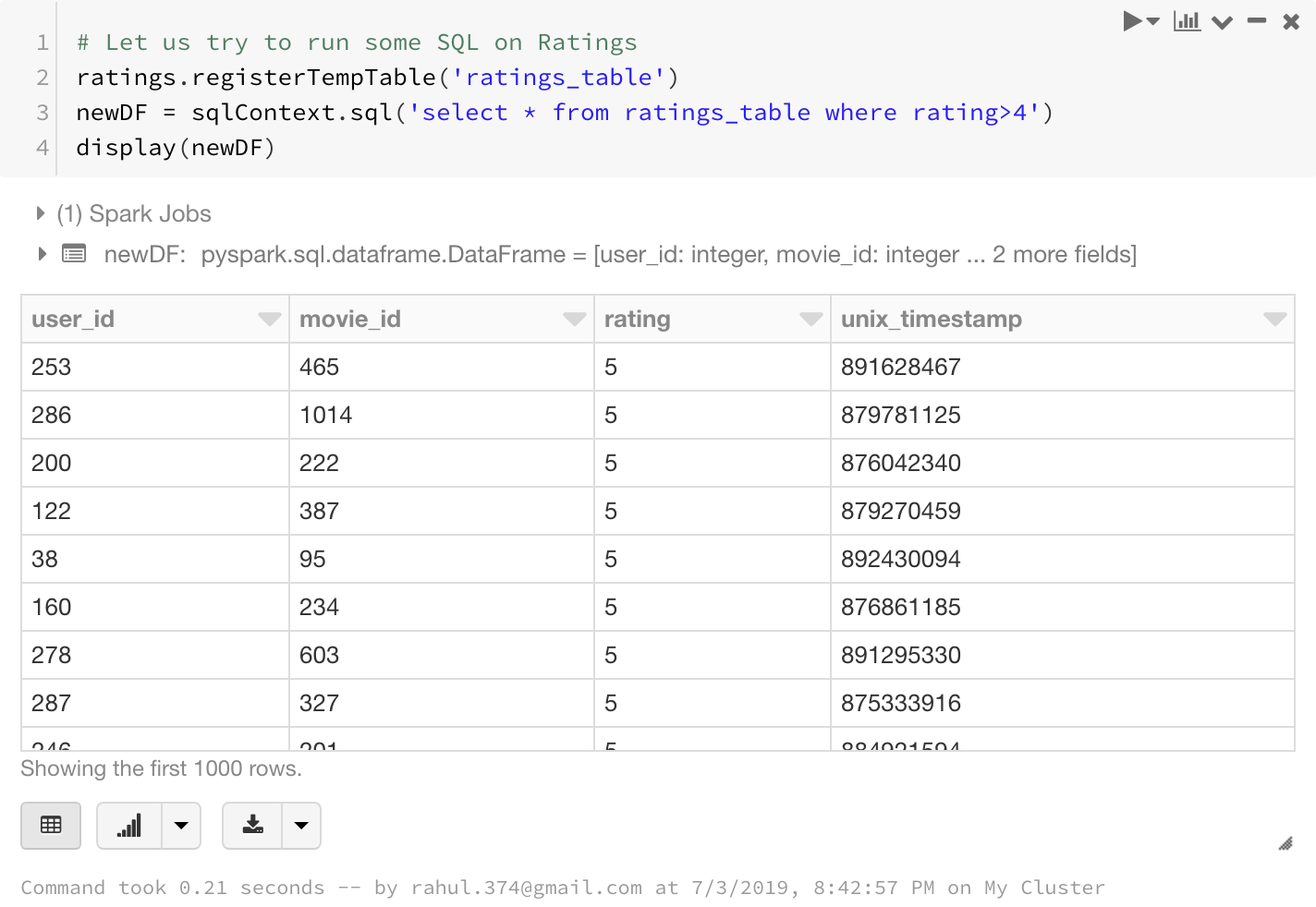
Let us try to run some SQL on Ratings.

We first register the ratings df to a temporary table ratings_table on which we can run sql operations.

As you can see the result of the SQL select statement is again a Spark Dataframe.

ratings.registerTempTable('ratings_table')
newDF = sqlContext.sql('select * from ratings_table where rating>4')
display(newDF)

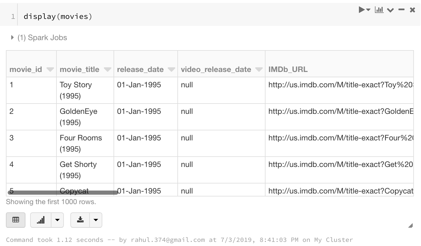
Let us now add one more Spark Dataframe to the mix to see if we can use join using the SQL queries:

#get one more dataframe to join
movies = spark.read.load("/FileStore/tables/u.item",format="csv", sep="|", inferSchema="true", header="false")

# change column names
movies = movies.toDF(*["movie_id","movie_title","release_date","video_release_date","IMDb_URL","unknown","Action","Adventure","Animation ","Children","Comedy","Crime","Documentary","Drama","Fantasy","Film_Noir","Horror","Musical","Mystery","Romance","Sci_Fi","Thriller","War","Western"])

display(movies)

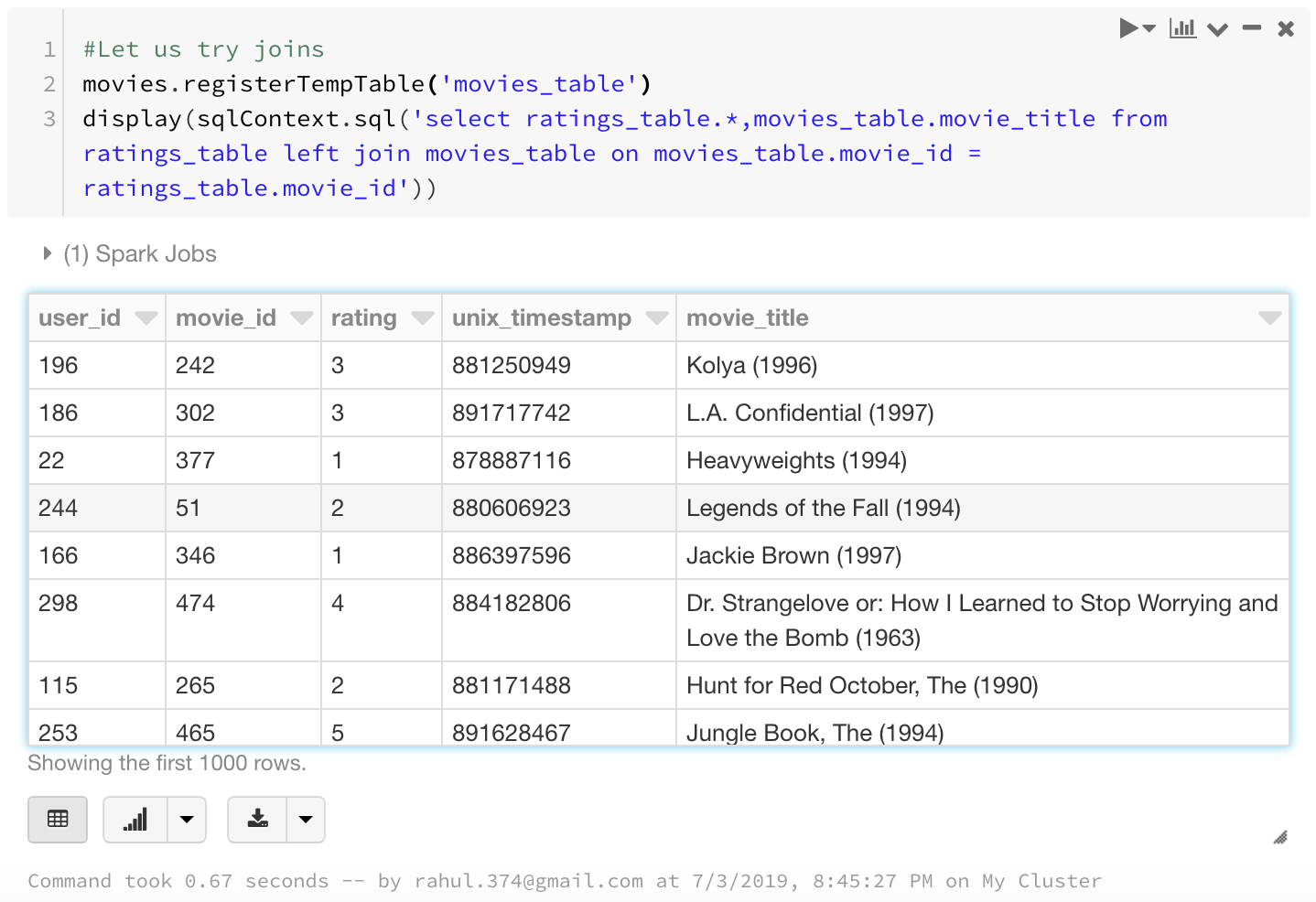
Now let us try joining the tables on movie_id to get the name of the movie in the ratings table.

movies.registerTempTable('movies_table')

display(sqlContext.sql('select ratings_table.*,movies_table.movie_title from ratings_table left join movies_table on movies_table.movie_id = ratings_table.movie_id'))

Let us try to do what we were doing earlier with the RDDs. Finding the top 25 most rated movies:

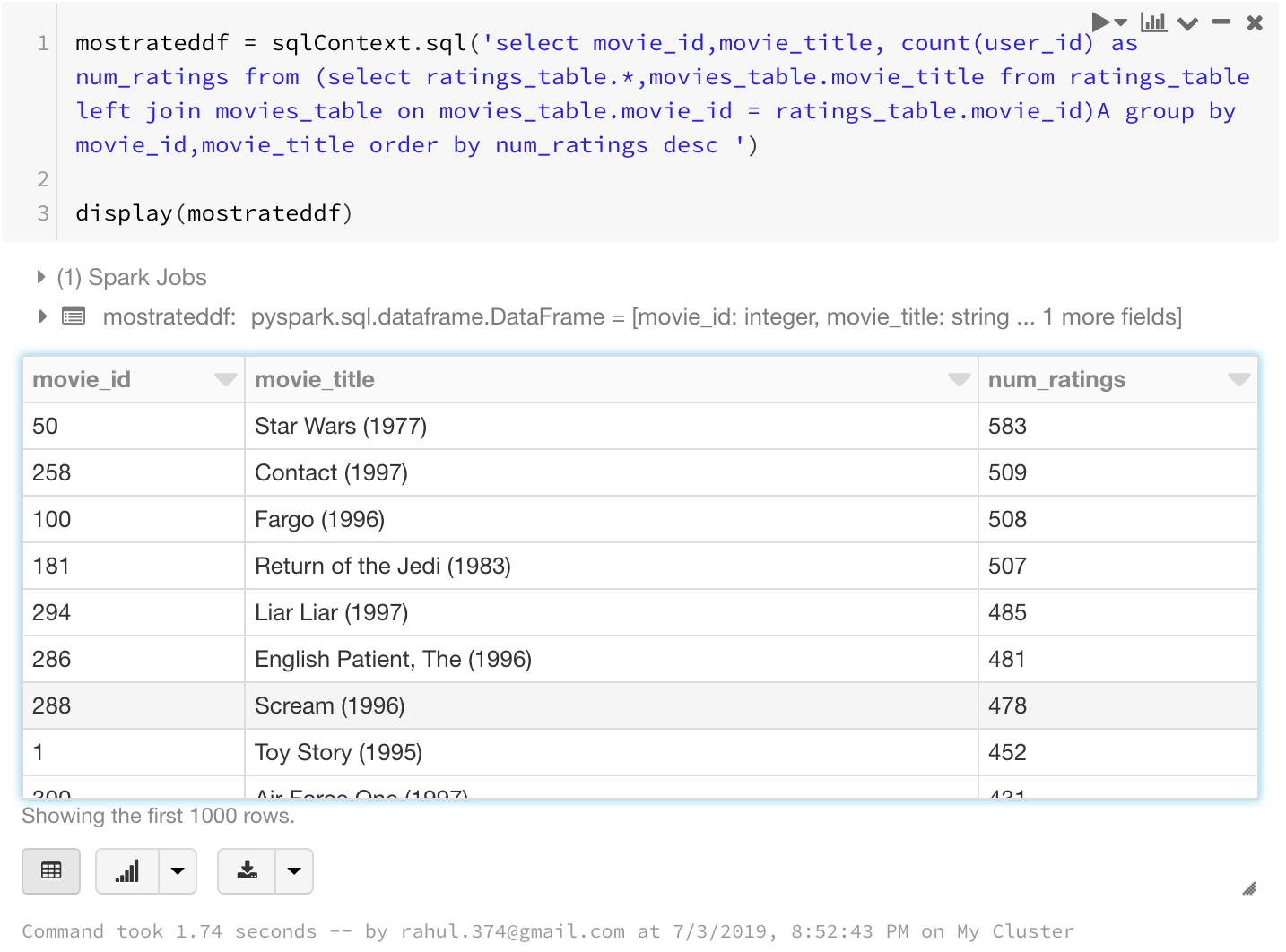
mostrateddf = sqlContext.sql('select movie_id,movie_title, count(user_id) as num_ratings from (select ratings_table.*,movies_table.movie_title from ratings_table left join movies_table on movies_table.movie_id = ratings_table.movie_id)A group by movie_id,movie_title order by num_ratings desc ')

display(mostrateddf)

And finding the top 25 highest rated movies having more than 100 votes:

highrateddf = sqlContext.sql('select movie_id,movie_title, avg(rating) as avg_rating,count(movie_id) as num_ratings from (select ratings_table.*,movies_table.movie_title from ratings_table left join movies_table on movies_table.movie_id = ratings_table.movie_id)A group by movie_id,movie_title having num_ratings>100 order by avg_rating desc ')

display(highrateddf)

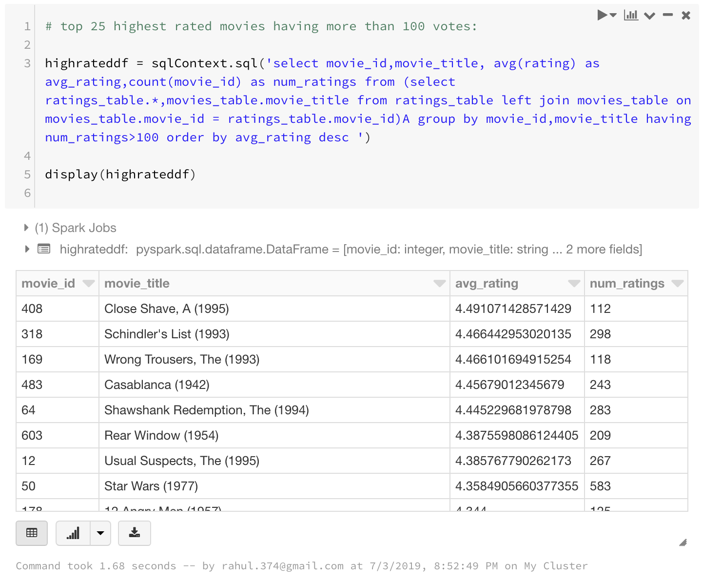
I have used GROUP BY, HAVING, AND ORDER BY clauses as well as aliases in the above query. That shows that you can do pretty much complex stuff using sqlContext.sql

A Small Note About Display

You can also use display command to display charts in your notebooks.

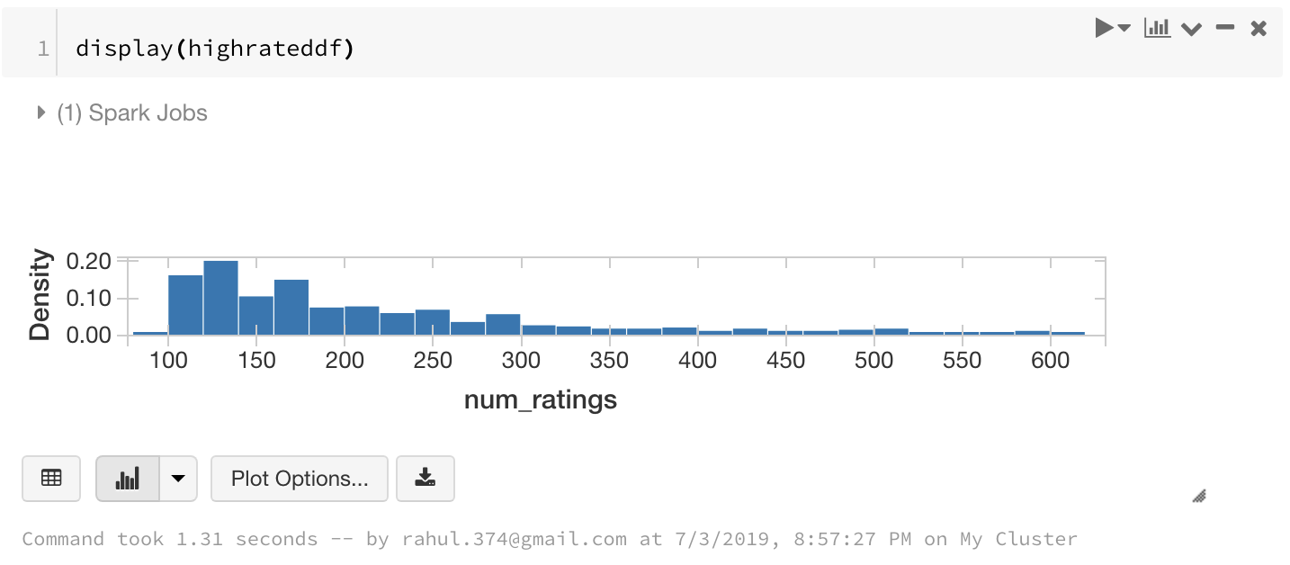
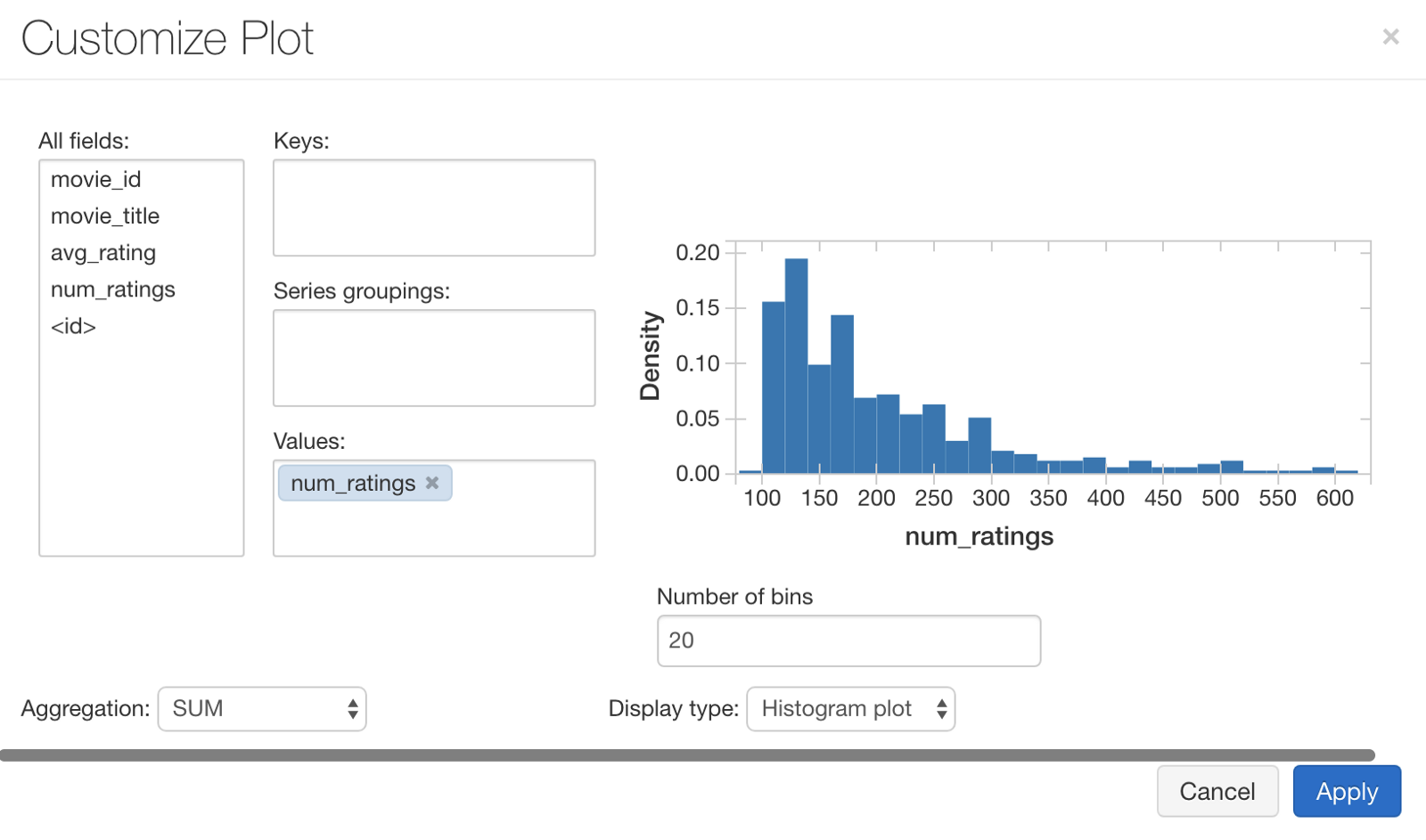
You can see more options when you select Plot Options.

Converting from Spark Dataframe to RDD and vice versa:

Sometimes you may want to convert to RDD from a spark Dataframe or vice versa so that you can have the best of both worlds.

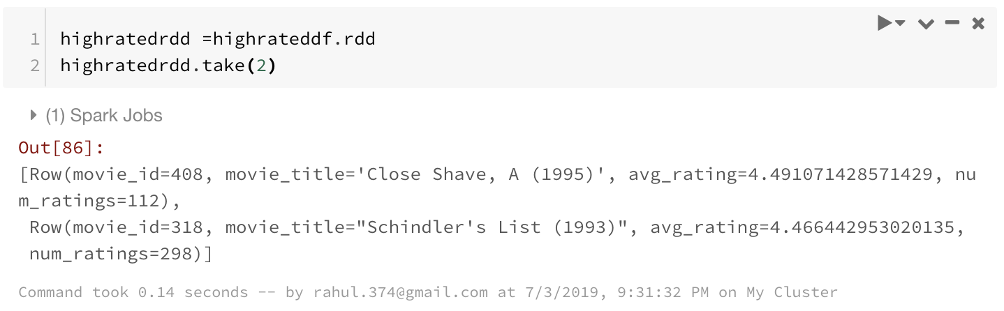
To convert from DF to RDD, you can simply do :

highratedrdd =highrateddf.rdd
highratedrdd.take(2)

To go from an RDD to a dataframe:

from pyspark.sql import Row
# creating a RDD first
data = [('A',1),('B',2),('C',3),('D',4)]
rdd = sc.parallelize(data)

# map the schema using Row.
rdd_new = rdd.map(lambda x: Row(key=x[0], value=int(x[1])))

# Convert the rdd to Dataframe
rdd_as_df = sqlContext.createDataFrame(rdd_new)
display(rdd_as_df)

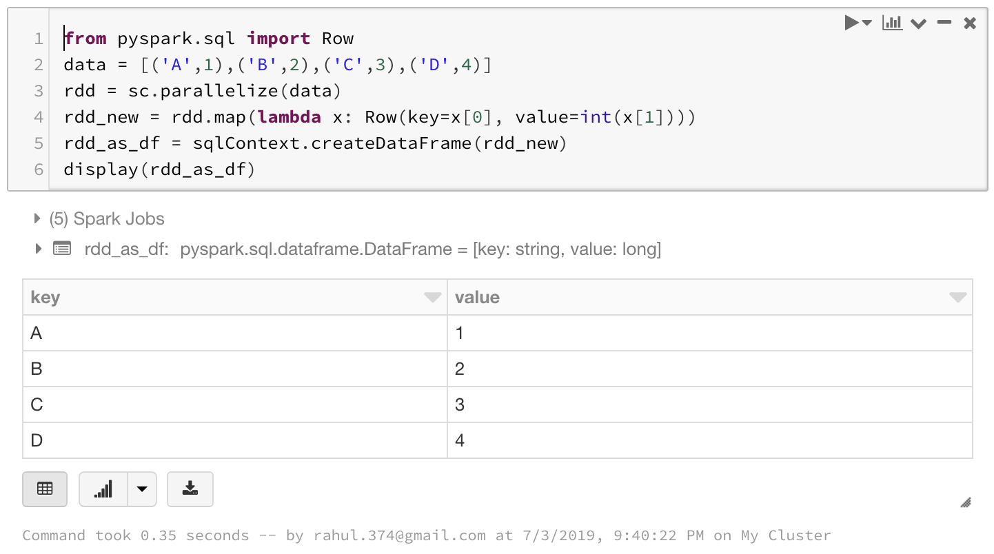
RDD provides you with more control at the cost of time and coding effort. While Dataframes provide you with familiar coding platform. And now you can move back and forth between these two.

Conclusion

This was a big post and congratulations if you reached the end.

Spark has provided us with an interface where we could use transformations and actions on our data. Spark also has the Dataframe API to ease the transition of Data scientists to Big Data.

Hopefully, I’ve covered the basics well enough to pique your interest and help you get started with Spark.

You can find all the code at the GitHub repository.

Also, if you want to learn more about Spark and Spark DataFrames, I would like to call out an excellent course on Big Data Essentials: HDFS, MapReduce and Spark RDD on Coursera.

I am going to be writing more of such posts in the future too. Let me know what you think about the series. Follow me up at <strong>Medium</strong> or Subscribe to my <strong>blog</strong> .